III. Vertical Heat Flux

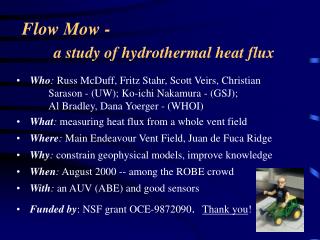
1. 250 200 CTD 150 ABE 100 50 Bathymetric contour interval: 100m SAS N 2000 MEF ‘95 S 2000 Current Meters LOW BUOYANCY FLUX FIELDS: C = Cirque D = Dune CB = Clam Bed Q = Quebec HIGH BUOYANCY FLUX FIELDS: SAS = Sasquatch SDF = Salty Dawg HRF = High Rise MEF = Main Endeavour MF = Mothra Recently discovered fields <Dq>N=0.051 oC <Dq>S=0.047 oC Ridge crests ABE survey Htop Ridge crest Hsides 2100 2200 mab Sea floor Depth HhighB HlowB OS21B-0444 Measurements and Models of Heat Flux Magnitude and Variance from the Main Endeavour Hydrothermal Vent Field Scott R. Veirs, Fritz R. Stahr, Russell E. McDuff, Richard E. Thomson, Dana R. Yoerger, and Albert M. Bradley School of Oceanography, University of Washington, Box 357940, Seattle, WA, 98195-7940 | scottv@ocean.washington.edu | www2.ocean.washington.edu/~scottv/ III. Vertical Heat Flux I. Background II. Lateral Heat Flux Method of calculation: Htop = r Cp A (1/N) [(Dq - <Dq>S ) w][Watts] Area (A) is the survey coverage (300m x 720m). <Dq>S characterizes entrained fluid that was advected into the field from the south. Vertical velocity (w) derives from MAVS minus ABE or from a dynamic model of ABE’s response to vertical advection within plumes. Mean r and Cp of each top is used. Summation is over all points of ABE’s trackline. The Flow Mow Experiment: In August 2000, we measured the flux of heat through a control volume enclosing the Main Endeavour hydrothermal vent field (MEF). Vertical flux was monitored ~75m above the vents with a CTD and acoustic velocity sensor (MAVS) mounted on the Autonomous Benthic Explorer (ABE). Lateral heat flux was estimated by combining ABE data, CTD observations, and current meter records acquired near the MEF and close to the seafloor. Methodology: Because southward tidal displacement rarely exceeds 50m, the south side of the control volume is usually colder than the north side. The mean Dq from any side can be multiplied by the orthogonal component of velocity (v), as well as density (r), heat capacity (Cp), and area (A), to estimate the heat flux (H) through that surface: ABE dive 50 MEF perimeter Dq : North side oC South side H = r Cp Dq A v Magnitude and variance: Pooling and streaming cause high variance : Periods when currents stream steadily through the control volume are times when heat flux can be estimated accurately by differencing the flux through opposite sides. But warmed fluid pools within the MEF during almost every tidal cycle. We use a numerical “puff” model to generate time series of flux through any side of the MEF and understand the high variance in the observed Dq and v (below). ABE surveyed the top of the MEF control volume 15 times; 12 of these “tops” led to robust estimates of Htop. The magnitude of each is shown here versus the mid-point of dive time. (Note that dives 44, 50 and 51 included multiple tops.) The black line is the mean for the experiment: 524 MW. Local currents and hydrography: Within the Endeavour segment’s axial valley (>2100m depth), currents are dominated by semidiurnal oscillations superimposed on a mean northward ~2-4cm/s flow. Please refer to the gentleman shown at left (Rick Thomson) for further details... South North South of MEF: North of MEF: Variance of observations: σ = 236.3 MW Variance of mean: [σ / (12)1/2] = 65.3 MW Observed magnitude and modeled variance: Each heat flux value below is estimated by multiplying a mean velocity by the mean Dq difference between N and S sides of the field (<Dq >N- <Dq >S ). Modeled variance for each current meter record is given at right. IV. Heat Budget Implications HhighB + HlowB + Htop + Hsides= 0 HlowB = Htop + Hsides - HhighB ~ 520 +100 -340* = 280 MW therefore, HlowB ~ HhighB ~ 300 MW * ~mean HhighB from Bemis et al (1993) and Ginster et al (1994) Simulated MEF Hsides Proximity of Dq observations to MEF: near ABE50 distant all <Dq >N- <Dq >S [oC] Velocity data sourceduration<v> (cm/s) 0.025 0.02 0.002 0.004 South mooring 2168 74 days1.6 27 22 2.2 4.4 South, survey only 17 days 1.1 24 19 1.9 3.8 North WASP 2161 142 days 4.1 91 73 7.3 15 North, survey only 17 days 5.1 114 91 9.1 18.2 North, ABE dive 50 only ~1 day 6.1 109 South, ABE dive 50 only ~1 day 3.9 70 Notes:r~1037.5; Cp~3800; A=300m x 75m [MW] Histograms of mean potential temperature anomaly (Dq ) within different depth bins reveal that fluid confined by the axial valley is warmer north of the MEF than to the south. The variance of Dq at these depths also increases to the north. A simple explanation for this near-bottom hydrography is that the mean flow transports MEF heat northward within the valley while tidal oscillations enhance variability. Normalized horizontal heat flux