Download
1 / 25
280 likes | 492 Views
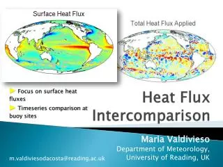
Heat Flux Intercomparison. ▶ Focus on surface heat fluxes ▶ Timeseries comparison at buoy sites . Maria Valdivieso Department of Meteorology, University of Reading, UK . m.valdiviesodacosta@reading.ac.uk. Monthly mean data regridded onto the WOA grid Common period 2004 – 2009

E N D
Heat Flux Intercomparison ▶Focus on surface heat fluxes ▶Timeseries comparison at buoy sites Maria Valdivieso Department of Meteorology, University of Reading, UK m.valdiviesodacosta@reading.ac.uk
Monthly mean data regridded onto the WOA grid Common period 2004 – 2009 ▶Other flux data sets: ISCCP+OAFlux, NOC2.0, ERAI, NCEP –R2
Global Integrals Surface heat fluxes from ocean reanalysis products averaged over the global ocean (common ocean-land mask). Fluxes are positive into the ocean. Units are in Wm-2
◀ ◀ ◀ ◀ Fluxes are positive into the ocean. Units are in Wm-2
Zonal Integrals Mean 2004 - 09
Zonal Integrals Equatorial heating in the middle of the range span by other products Warming pattern in the SH underestimated at all latitudes Heat loss north of 20N seems reasonable
Mean 2004 - 09 Northward heat transport - global MHT as inferred from estimated surface heat fluxes The mean transport due to the net heat uptake is ~ 2 PW, representing a non-zero heat storage in these ocean reanalyses Also shown are the zonal integrals from Ganachaud and Wunsch (2003) and Lumpkin and Speer (2007) obtained from inverse analysis of WOCE sections
Differences in Qsw Mean 2004 - 09 Atmos reanalysis Satellite-based Cloud estimation from ships Coupled reanalysis Global averages over 2004 –2009. Units in Wm-2
Mean 2004 - 09 SST Diff Maps HadISST (Rayner et al., 2003) combines in situ + satellite-based data Using COREII surface fields JMA Reanalysis surface fields Using NCEP-R2 + relaxation to weekly OISST Using NCEP surface fields
Using corrected ERAI Qsw SST Diff Maps (cont.) Mean 2004 - 09 Coupled Reanalyses Assimilating Reynolds SSTs OSTIA + real time GHRSST after 2008
Mean 2004 - 09 Differences in the bulk fluxes Eddy-permitting + Core bulk forcing using ERAI surface fields No data assimilation Assimilating SST + CORA data Assimilating EN3 T/S profiles Assimilating SST + EN3 data
Comparison at buoy sites CLIMODE: 38.5N, 65W KEO: 32.4N, 144.5E WHOTS: 22N, 158W NTAS: 15N, 51W TAO_w: 0, 165E TAO_e: 0, 110W STRATUS: 25S, 85W The underlying map is the annual mean (1993 – 2009) net surface heat flux from the OAFlux + ISCCP product (Wm-2, positive downward) available at http://oaflux.whoi.edu
Monthly Climatology 2004 - 2009 CLIMODE [38.5N, 65.0W] Mean (ISCCP+OAF) = -206.4 ±22.4 Wm-2
Sea Surface Temperatures warm winters in 2008 and 2009 Monthly Climatology 2004 - 2009 Interestingly, GODAS net heat flux is much too weak here (only -47 Wm-2), yet the SST is reasonably well reproduced. GECCO2 is systematically too cold; MOVECORE is too warm
KEO [32.4N, 144.5E] Mean (ISCCP+OAF) = -101.35 ±16.2 Wm-2
WHOTS • [22.0N, 158.0W] Mean (ISCCP+OAF) = +23.53 ± 9.96 Wm-2
Sea Surface Temperatures Surface Heat Fluxes
NTAS • [15N, 51W] Mean (ISCCP+OAF) = +40.25 ± 8.2 Wm-2
STRATUS • [25S, 85W] Mean (ISCCP+OAF) = +52.56 ±8.83 Wm-2
Sea Surface Temperatures Surface Heat Fluxes
TAO_w • [0, 165E] Mean (ISCCP+OAF) = +56.68 ±21.62 Wm-2
TAO_e • [0, 110W] Mean (ISCCP+OAF) = +157.8 ± 9.86 Wm-2
Mean (2004 -09) differences at buoy sites For CLIMODE, the overall biases (less cooling) result primarily from the winter months. Here, fluxes are sensitive to the model resolution. In the central tropical Pacific (WHOTS) and tropical Atlantic (NTAS), fluxes show less warming during spring and summer. In the south east Pac (STRATUS), fluxes show less warming in the summer months and more cooling in the winter. For TAO locations, fluxes provide less warming all year round. KEO, for the Kuroshio region, and TAO_w have the smallest differences. Ocean Reana Based minus ISCCP+OAFlux ISCCP + OAFlux versus Ocean Reanalyses
Comparing with other flux products Ocean Reana Based minus ISCCP+OAFlux Mean Differences Product - (ISCCP + OAFlux)
Summary Most ocean reanalysis show a positive imbalance in global surface heating (ensemble mean of ~ 4 Wm-2 over 1993-2009). This can be as large as 14 Wm-2 in coupled reanalyses. Generally, the imbalance is reduced as more observations become available after 2004. Ocean reanalysis-based fluxes are biased low compared to ISCCP+OAFlux data at all buoy locations. Variability is generally well reproduced. The result that the reanalysis SSTs compare reasonably well with HadISST data while the reanalysis-based fluxes are systematically too low compared to ISCCP+OAFlux data suggests that the models stratify the upper ocean too strongly. This may be a result of inadequate vertical mixing, weak advection, ... Direct flux measurements are needed for further validation.


![Heat Flux [Wm -2 ]](https://cdn3.slideserve.com/5899967/heat-flux-wm-2-dt.jpg)