Sensible heat flux
430 likes | 1.3k Views
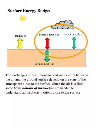
Latent heat flux. Sensible heat flux. Radiation. Ground heat flux. Surface Energy Budget.

Sensible heat flux
E N D
Presentation Transcript
Latent heat flux Sensible heat flux Radiation Ground heat flux Surface Energy Budget The exchanges of heat, moisture and momentum between the air and the ground surface depend on the state of the atmosphere close to the surface. Since the air is a fluid, some basic notions of turbulence are needed to understand atmospheric motions close to the surface.
Viscous fluids The viscosity causes an irreversible transfer of momentum from the points where the velocity is large to those where it is small. It is an internal resistance of fluid to deformation In 1D The momentum flux density t (also called shearing stress) due to viscosity is proportional to the gradient of the velocities. m is called the dynamic viscosity and it is a property of the fluid.
Generalizing in three dimensions Only for people interested in the mathematical approach
is a momentum flux density, so its dimensions should be those of momentum (M L T-1), per unit time (T-1) , per unit surface (L-2). As a consequence, the dimensions of m are L=length T=time M=mass So the units of m are kg m-1 s-1 The ratio v=m/r is called kinematic viscosity (units m2 s-1).
Fluid particle of a viscous fluid adhere to solid surface. If the surface is at rest, the fluid motion right at the surface must vanish (No slip boundary condition). Viscosity dissipates kinetic energy of the fluid motion. Kinetic energy is converted to heat. To maintain the motion, the energy has to be continuously supplied externally, or converted from potential energy, which exist in the form of pressure and density gradients in the flow.
Osborne Reynolds (English, 1842-1912): “The internal motion of water assumes one or other of two broadly distinguishable forms – either the elements of the fluid follow one another along lines of motion which lead in the most direct manner to their destination, or they eddy about in sinuous paths the most indirect possible” “Laminar” “Turbulent”
In which conditions the flow is laminar and in which turbulent ? Reynolds made an experiment the 22nd of February 1880 (at 2 pm). He varied the speed of the flow, the density of the water (by varying the water temperature), and the diameter of the pipe. He used colorants in the water to detect the transition from Laminar to Turbulent.
He found that when The flow becomes turbulent More in general, the ratio with L typical length scale of the flow, is called “Reynolds number”. The critical value of the transition from laminar to turbulent flow changes with the type of flow
Reynolds number is very important in fluid mechanics The flow behaves in two different ways for low and high Reynolds numbers. For Low Reynolds numbers the flow is Laminar A laminar flow is characterized by smooth, orderly and slow motions. Streamlines are parallel and adjacent layers (laminae) of fluid slide past each other with little mixing and transfer (only at molecular scale) of properties across the layers. A small perturbation does not increase with time. The flow is regular and predictable.
For high Reynolds numbers the flow is turbulent Turbulent flows are highly irregular, three-dimensional, rotational, and very diffusive and dissipative. A small perturbation increases with time. They cannot be predicted exactly as function of time and space. Only statistical averaged variables can be predicted.
Physical meaning of the Reynolds number Newton’s second Law For a fluid parcel It links the acceleration of a fluid parcel, with the forces acting on the parcel. Since momentum is conserved, you can think at the Newton’s second law as a budget equation. If the sum (in vector sense) of all the forces acting on a parcel is different than zero, there is a change in momentum.
For example, for u (x component) of the wind vector (but similar reasoning can be done for the others components) Term of Inertia. If the others terms are zero, the air parcel keeps moving at the same speed Pressure forces (we’re not interested at this moment) Viscous forces. This can be seen also as budget (input-output) of momentum fluxes induced by viscosity We focus only on the inertia and viscous terms
If U is a characteristics velocity of the flow, and L a characteristic length, a characteristic time can be deduced from U=L/T Inertial term Viscous term The ratio between the inertial and the viscous term give the relative importance of one respect to the other This is the Reynolds number
A high Reynolds number means that the inertial terms in the equation of motion are far greater than the viscous terms. However, viscosity cannot be neglected, because of the no-slip boundary condition at the interface.
The value of the critical Reynolds number (for the transition from laminar to turbulent flows) varies a lot from one case to the other (between 103 and 105). However in the atmosphere typical values are between 106 and 109. Atmosphere is turbulent Moreover, in the generation or damping of turbulence in the atmosphere a very important role is played by the buoyancy effects (we will see later on).
Properties of turbulence Irregularity or randomness Highly sensitive to small perturbations (changes in initial and boundary conditions). Unpredictable. Only statistical description can be used.
Three dimensionality and rotationality The velocity field in any turbulent flow is three-dimensional, and highly rotational.
Diffusivity or ability to mix properties Very efficient in diffuse momentum, heat and mass. “Macroscale” diffusivity of turbulence is usually many order of magnitude larger than the molecular diffusivity. This is one of the most important properties concerning the applications. It is largely responsible of the dispersion of pollutants
Multiplicity of scales of motion and dissipativeness Turbulent flows are characterized by a wide range of scales. The energy is transferred from the mean flow, to the larger eddies. There is a continuous transfer of energy from the largest to the smallest eddies. Viscous dissipation of energy occurs in the smallest eddies. In order to maintain the turbulent motion energy must be supplied continuously. Energy dissipated
Mean and fluctuating variables It is useful to split a variable in “mean” and “fluctuating” part Wind velocity time Only averaged values of turbulent flows are predictable. Instantaneous values are random.
For example for the three wind components (u_> x, or West-East direction, v-> y or South-North direction, w _> z or bottom-up direction) Reynolds decomposition In the analysis of observations the most common mean or average used is the time average. For a generic variable f For micrometeorological observations, the averaging time T ranges between 103 and 104.
In modeling, more used are spatial averages Average value over a grid cell Dz Dy Dx In some cases a spatial and time average is also performed. In micro- and meso- scale simulations, Dx and Dy range between 102 and 103. Dz near the surface is between 10 and 102
In laboratory and some modeling and theoretical studies the ensemble average is used. This is an arithmetical average over a very large (approaching infinite) number of realization of a variable, obtained by repeating the experiment over and over again under the same general conditions. Nearly impossible to do in real atmospheric conditions Theoretically the three averages are equal only for homogeneous and stationary flows. These conditions are very difficult to satisfy in micrometeorological applications. However, very often it is expected that an approximate correspondence between the results of the three averages exists.
So, by definition It is assumed that the average operator is such that the average of the fluctuations is zero. For the product of two variables
Ds uDt Co-variances or turbulent fluxes Let consider a quantity c(per unit volume, ex: Mass per unit volume= density). If it is only transported, its flux density is a function of the wind speed Splitting in mean and turbulent part and averaging The term Is the the covariance, and represent the turbulent flux density
For the momentum These are called Reynolds stress, and they are much larger in magnitude than the correspondent viscous stress The ratio is proportional to the Reynolds number Turbulent mixing is much more efficient than viscous mixing
Variances are the simplest measure of the fluctuations s are also called standard deviations. The ratio of standard deviations over mean wind speed are called turbulence intensities. In the atmosphere, turbulence intensities are less than 10% in the nocturnal boundary layer, 10-15% in a near-neutral surface layer, and greater than 15% in a unstable and convective boundary layers.
By combining the variances, it is possible to estimate the kinetic energy of the turbulent part, or Turbulent Kinetic Energy (TKE) per unit mass. The kinetic energy of the flow is the sum of the Mean Kinetic Energy (MKE) and the Turbulent Kinetic Energy (TKE). KE=MKE+TKE


![Heat Flux [Wm -2 ]](https://cdn3.slideserve.com/5899967/heat-flux-wm-2-dt.jpg)