Download
1 / 21
210 likes | 315 Views
Study on seabird diet composition using a latent Gaussian model for zero-inflated data, analyzed with Approximate Bayesian Computation (ABC) methods.

E N D
A latent Gaussian model for compositional data with structural zeroes Adam Butler & Chris Glasbey Biomathematics & Statistics Scotland
1. Application to seabird diet • How does the composition of seabirddiet vary between colonies, years and seasons…? • Kittiwake data from four islands on the East coast of Scotland for 1997-2000 • Previously analysed byBull et al. (2004)
Relative proportions of D=3 food types: - SE0: juveline sandeels - SE1: adult sandeels - Other species (aggregated) • 543 individual birds – • 251 have SE0 only • 51 have SE1 only • 80 have “other” only • 158 have a mix
2. Compositional data • Compositional data refer to relative frequencies (proportions), and frequently arise in fields such as geology, economics and ecology. • If x denote data on the proportions of D components then x must lie on the unix simplex: • Such data cannot be analysed using standard methods because of the sum constraintthat xT1 = 1.
Well established approach for dealing with compositional data by modelling log-ratios of x using a multivariate normal distribution: Aitchison (1986) • If x lies on the interior of the simplex this works well, but it cannot be applied when some proportions of x are zero • No general approach for situation in which zero values of x may correspond to genuine absences of a component: “structural zeroes”
We assume that x=g(y), where: • y has a D-dimensional multivariate normal distribution with mean and covariance matrix , where T1=1 and 1=0. • g is the function which performs a Euclidean projection of yonto the unit SimplexSD
Parsimonious: (D-1)(D+2)/2 parameters • Relatively flexible– can cope with a high proportion of zero values • No mathematical justification for our model, so important to check fit to the data • Diagnostic: compare patterns of zero values in the data with those given by the model
4. Inference • The log-likelihood function is • where: D(x;,)is the PDF of a multivariate normal distribution • is the “inverse” of g(y)
For general D the likelihood cannot be evaluated analytically, because: • There are no explicit formulae for either g(y) or h(x) • If we could evaluate h(x) the likelihood would still contain intractable integrals…
But in order to simulate from the model we only need to find the Euclidean projection of y onto the unit simplex: • We propose an iterative algorithm for doing this – will reach solution in at most D-1 steps
5. Approximate Bayesian Computation “ABC” is a methodology for drawing inferences by Monte Carlo simulation when the likelihood is intractable but the model is easy to simulate from In usual MCMC we tend to accept parameter values that have relatively high values of the likelihood In ABC we tend to accept parameter values that simulate data with summary statistics similar to those of the real data
Elements of ABC: Prior distribution() Summary statisticsS, Distance measure, threshold Number of samplesN
Basic ABC algorithm: for (i = 1,…,N) { (1) Generate values *by simulating from prior () (2) Simulate y*from model with parameters * (3) If D(S(y*), S(y)) < then set (i) = *; else go to (1) }
Generate values {0(1),…,0(N)}by simulating from prior () and applying basic ABC algorithm with threshold e0 for (t = 1,…,T) { Generate values {t(1),…,t(N)}by sampling from {t-1(1),…,t-1(N)}, proposing a move using q, and applying basic ABC algorithm with threshold et } Take et = , need proposal distn q,thresholdse0, e0,…,eT-1 Sequential ABC algorithm (Sisson et al., 2006)
Elements of ABC – our choices: Prior distribution(): uniform over a wide interval Summary statisticsS: - marginal means, marginal variances (x2); - means of differences between components (/2); - proportions of zero and one values for each component Distance measure D: Mean of absolute values of the elements of S(y*) - S(y)
6. Results – simulated data D=3 components Compare ABC (black) and analytic MLEs (red) Generate n=200 obs from symmetric model with marginal SDs of 1
6. Results – seabird data Aim in future to apply model to: - individual groups - more diet classes
7. Conclusions • Parsimonious model for compositional data that contain structural zeroes • Developed an iterative algorithm to simulate from the model • Likelihood cannot be computed analytically, so use ABC methods to draw inferences • Sequential ABC algorithm (Sisson et al., 2006) much more efficient than other ABC algorithms
Further information Email: adam@bioss.ac.uk Manuscript: www.bioss.ac.uk/staff/adam/publications.html http://www.rolexawards.com/special-feature/creatures/img/large506.jpg