Modeling compositional data
Modeling compositional data. Some collaborators. Deformations: Paul Sampson Wendy Meiring, Doris Damian Space-time: Tilmann Gneiting Francesca Bruno Deterministic models: Montserrat Fuentes, Peter Challenor Markov random fields: Finn Lindstr ö m Wavelets: Don Percival


Modeling compositional data
E N D
Presentation Transcript
Some collaborators • Deformations: Paul Sampson • Wendy Meiring, Doris Damian • Space-time: Tilmann Gneiting • Francesca Bruno • Deterministic models: Montserrat Fuentes, Peter Challenor • Markov random fields: Finn Lindström • Wavelets: Don Percival • Brandon Whitcher, Peter Craigmile, Debashis Mondal
Background • NAPAP, 1980’s • Workshop on biological monitoring, 1986 • Dirichlet process: Gary Grunwald, 1987 • Current framework: Dean Billheimer, 1995 • Other co-workers: Adrian Raftery, Mariabeth Silkey, Eun-Sug Park
Compositional data • Vector of proportions • Proportion of taxes in different categories • Composition of rock samples • Composition of biological populations • Composition of air pollution
The triangle plot 1 Proportion 1 (0.55,0.15,0.30) 0 0 Proportion 2 1 1 0 Proportion 3
The spider plot 0.2 0.4 0.6 0.8 1.0 (0.40,0.20,0.10,0.05,0.25)
An algebra for compositions • Perturbation: For define • The composition acts as a zero, so . • Set so . • Finally define .
The logistic normal • If • we say that z is logistic normal, in short Z ~ LN(m,S). • Other distributions on the simplex: • Dirichlet — ratios of independent gammas • “Danish” — ratios of independent inverse Gaussian • Both have very limited correlation structure.
Scalar multiplication • Let a be a scalar. Define • is a complete inner product space, with inner product given, e.g., by • N is the multinomial covariance N=I+jjT • j is a vector of k-1 ones. • is a norm on the simplex. • The inner product and norm are invariant to permutations of the components of the composition.
Some models • Measurement error: • where ej ~ LN(0,S) . • Regression: • Correspondence in Euclidean space: • xjxg uj centered covariate compositions
A source receptor model • Observe relative concentration Yi of k species at a location over time. • Consider p sources with chemical profiles qj. Let ai be the vector of mixing proportions of the different sources at the receptor on day i. • Q ~ LN, ai ~ indep LN, ei ~ zero mean LN
Juneau air quality • 50 observations of relative mass of 5 chemical species. Goal: determine the contribution of wood smoke to local pollution load. • Prior specification: • Inference by MCMC.
Wood smoke contribution 95% CL 50% CL
Source profiles (pyrene) (benzo(a)) (fluoranthene) (chrysene) (benzo(b))
State-space model • Space-time model of proportions • State-space model: • zj unobservable composition ~ LN(mj,Sj) • yj k-vector of counts ~ Mult( • Inference using MCMC again
Stability of arthropod food webs • Omnivory thought to destabilize ecological communities • Stability: Capacity to recover from shock (relative abundance in trophic classes) • Mount St. Helens experiment: 6 treat-ments in 2-way factorial design; 5 reps. • Predator manipulation (3 levels) • Vegetation disturbance (2 levels) • Count anthropods, 6 wks after treatment. Divide into specialized herbivores, general herbivores, predators.
Specification of structure • is generated from independent observations at each treatment • mean depends only on treatment
Benthic invertebrates in estuary • EMAP estuaries monitoring program: Delaware Bay 1990. 25 locations, 3 grab samples of bottom sediment during summer • Invertebrates in samples classified into • pollution tolerant • pollution intolerant • suspension feeders (control group; mainly palp worms)
Site j, subsample t • qj ~ CAR process