Gaussian Process Structural Equation Models with Latent Variables
520 likes | 728 Views
Gaussian Process Structural Equation Models with Latent Variables. Ricardo Silva Department of Statistical Science University College London Robert B. Gramacy Statistical laboratory University of Cambridge. ricardo@stats.ucl.ac.uk. bobby@statslab.cam.ac.uk. Summary.

Gaussian Process Structural Equation Models with Latent Variables
E N D
Presentation Transcript
Gaussian Process Structural Equation Models with Latent Variables Ricardo SilvaDepartment of Statistical Science University College London Robert B. Gramacy Statistical laboratory University of Cambridge ricardo@stats.ucl.ac.uk bobby@statslab.cam.ac.uk
Summary • A Bayesian approach for graphical models with measurement error • Model: nonparametric DAG + linear measurement model • Related literature: structural equation models (SEM), error-in-variables regression • Applications: dimensionality reduction, density estimation, causal inference • Evaluation: social sciences/marketing data, biological domain • Approach: Gaussian process prior + MCMC • Bayesian pseudo-inputs model + space-filling priors
Measurement Error Problems Calorie intake Weight
Measurement Error Problems Calorie intake Reported calorie intake Weight Notation corner: Observed Latent
Error-in-variables Regression • Task: estimate error and f() • Error estimation can be treated separately • Caveat emptor: outrageously hard in theory • If errors are Gaussian, best (!) rate of convergence is O((1/log N)2), N sample size • Don’t panic Calorie intake Reported calorie intake = Calorie intake + error Weight = f(Calorie intake) + error Reported calorie intake Weight (Fan and Truong, 1993)
Error in Response/Density Estimation Calorie intake Weight Reported calorie intake Reported weight
Multiple Indicator Models Calorie intake Weight Self-reported calorie intake Weight recorded in the morning Assisted report ofcalorie intake Weight recorded in the evening
Chains of Measurement Error Widely studied as Structural Equations Models (SEMs) with latent variables Calorie intake Weight Well-being Reported calorie intake Reported time to fall asleep Reported weight (Bollen, 1989)
Quick Sidenote: Visualization Industrialization Level 1960 DemocratizationLevel 1965 DemocratizationLevel 1960 GNP etc. GNP etc. Fairness of elections etc. GNP etc. Fairness of elections etc. GNP etc.
Quick Sidenote: Visualization (Palomo et al., 2007)
Traditional SEM • Some assumptions • assume DAG structure • assume (for simplicity only) no observed variable has children in the • Linear functional relationships: • Parentless vertices ~ Gaussian Xi = i0 + XTP(i)Bi + i Yj = j0 + XTP(j)j + j Notation corner: Y X
Our Nonparametric SEM: Likelihood Functional relationships:where each fi() belongs to some functional space. Parentless latent variables follow a mixture of Gaussians, error terms are Gaussian Xi = fi(XP(i)) + i Yj = j0 + XTP(j)j + j j ~ N(0, vj) i ~ N(0, vi)
Related Ideas • GP Networks (Friedman and Nachman, 2000): • Reduces to our likelihood for Yi = “Xi” • Gaussian process latent variable model (Lawrence, 2005): • Module networks (Segal et al., 2005): • Shared non-linearitiese.g., Y4 = 40+41f(IL) + error, Y5 = 50+51f(IL) + error • Dynamic models (e.g., Ko and Fox, 2009) • Functions between different data points, symmetry
Identifiability Conditions • Given observed marginal M(Y) and DAG, are M(X), {}, {v} unique? • Relevance for causal inference and embedding • Embedding: problematic MCMC for latent variable interpretation if unidentifiable • Causal effect estimation: not resolved from data • Note: barring possible MCMC problems, not essential for prediction • Illustration: • Yj = X1 + error, for j = 1, 2, 3; Yj = 2X2 + error, j = 4, 5, 6 • X2 = 4X12 + error
Identifiable Model: Walkthrough Assumed structure (In this model, regression coefficients are fixed for Y1 and Y4.)
Non-Identifiable Model: Walkthrough Assumed structure (Nothing fixed, and all Y freely depend on both X1 and X2.)
The Identifiability Zoo • Many roads to identifiability via different sets of assumptions • We will ignore estimation issues in this discussion! • One generic approach boils down to a reduction to multivariate deconvolutionso that the density of X can be uniquely obtained from the (observable) density of Y and (given) density of error • But we have to nail the measurement error identification problem first. Y = X + error Hazelton and Turlach (2009)
Our Path in The Identifiability Zoo • The assumption of three or more “pure” indicators: • Scale, location and sign of Xi is arbitrary, so fix Y1i = Xi + i1 • It follows that remaining linear coefficients inYji = 0ji + 1jiXi +ji are identifiable, and so is the variance of each error term Xi Y1i Y2i Y3i (Bollen, 1989)
Our Path in The Identifiability Zoo Select one pure indicator per latent variable to form set Y1 (Y11, Y12, ..., Y1L) and E1 ( 11, 12, ..., 1L) Fromobtain the density of X, since Gaussian assumption for error terms results in density of E1 being known Notice: since density of X is identifiable, identifiability of directionality Xi Xj vs. Xj Xi is achievable in theory Y1 = X + E1 (Hoyer et al., 2008)
Quick Sidenote: Other Paths • Three “pure indicators” per variable might not be reasonable • Alternatives: • Two pure indicators, non-zero correlation between latent variables • Repeated measurements (e.g., Schennach 2004) • X* = X + error • X** = X + error • Y = f(X) + error • Also related: results on detecting presence of measurement error (Janzing et al., 2009) • For more: Econometrica, etc.
Priors: Parametric Components • Measurement model: standard linear regression priors • e.g., Gaussian prior for coefficients, inverse gamma for conditional variance • Could use the standard normal-gamma priors so that measurement model parameters are marginalized • In the experiments, we won’t use such normal-gamma priors, though, because we want to evaluate mixing in general • Samples using P(Y | X, f(X))p(X, f(X)) instead of P(Y | X, f(X), )p(X, f(X))p()
Priors: Nonparametric Components • Function f(XPa(i)): Gaussian process prior • f(XPa(i)(1)), f(XPa(i) (2)), ..., f(XPa(i) (N)) ~ jointly Gaussian with particular kernel function • Computational issues: • Scales as O(N3), N being sample size • Standard MCMC might converge poorly due to high conditional association between latent variables
The Pseudo-Inputs Model • Hierarchical approach • Recall: standard GP from {X(1), X(2), ..., X(N)}, obtain distribution over {f(X(1)), f(X(2)), ..., f(X(N))} • Predictions of “future” observations f(X*(1)), f(X*(2)), ..., etc. are jointly conditionally Gaussian too • Idea: • imagine you see a pseudo training set X • your “actual” training set {f(X(1)), f(X(2)), ..., f(X(N))} is conditionally Gaussian given X • however, drop all off-diagonal elements of the conditional covariance matrix (Snelson and Ghahramani, 2006; Banerjee et al., 2008)
The Pseudo-Inputs Model: SEM Context Standard model Pseudo-inputs model
Bayesian Pseudo-Inputs Treatment • Snelson and Ghaharamani (2006): empirical Bayes estimator for pseudo-inputs • Pseudo-inputs rapidly amounts to many more free parameters sometimes prone to overfitting • Here: “space-filling” prior • Let pseudo-inputs X have bounded support • Set p(Xi) det(D), where D is some kernel matrix • A priori, “spreads” points in some hyper-cube • No fitting: pseudo-inputs are sampled too • Essentially no (asymptotic) extra cost since we have to sample latent variables anyway • Possible mixing problems? REFERENCES HERE
Demonstration • Squared exponential kernel, hyperparameterl • exp(–|xi – xj|2 / l) • 1-dimensional pseudo-input space, 2 pseudo-data points • X(1), X(2) • Fix X(1) to zero, sample X(2) • NOT independent. It should differ from the uniform distribution at different degrees according to l
More on Priors and Pseudo-Points • Having a prior • treats overfitting • “blurs” pseudo-inputs, which theoretically leads to a bigger coverage • if number of pseudo-inputs is “insufficient,” might provide some edge over models with fixed pseudo-inputs, but care should be exercised • Example • Synthetic data with quadratic relationship
Predictive Samples Sampling 150 latent points from the predictive distribution, 2 fixed pseudo-inputs (Average predictive log-likelihood: -4.28)
Predictive Samples Sampling 150 latent points from the predictive distribution, 2 fixed pseudo-inputs (Average predictive log-likelihood: -4.47)
Predictive Samples Sampling 150 latent points from the predictive distribution, 2 free pseudo-inputs with priors (Average predictive log-likelihood: -3.89)
Predictive Samples With 3 free pseudo-inputs (Average predictive log-likelihood: -3.61)
MCMC Updates • Metropolis-Hastings, low parent dimensionality ( 3 parents in our examples) • Mostly standard. Main points: • It is possible to integrate away pseudo-functions. • Sampling function values {f(Xj(1)), ... f(Xj(N))} is done in two-stages: • Sample pseudo-functions for Xj conditioned on all but function values • Conditional covariance of pseudo-functions (“true” functions marginalized) • Then sample {f(Xj(1)), ... f(Xj(N))} (all conditionally independent) (N = number of training points, M = number of pseudo-points)
MCMC Updates • When sampling pseudo-input variable XPa(i)(d) • Factors: pseudo-functions and “regression weights” • Metropolis-Hastings step: • Warning: for large number of pseudo-points, p(fi(d) | f\i(d), X) can be highly peaked • Alternative: propose and sample fi(d)() jointly
MCMC Updates In order to calculate the ratio iterativelyfast submatrix updates are necessary for to obtain O(NM) cost per pseudo-point, i.e., total of O(NM2)
Setup • Evaluation of Markov chain behaviour • “Objective” model evaluation via predictive log-likelihood • Quick details • Squared exponential kernel • Prior for a (and b): mixture of Gamma (1, 20) + Gamma(20, 20) • M = 50
Synthetic Example • Our old friend • Yj = X1 + error, for j = 1, 2, 3; Yj = 2X2 + error, j = 4, 5, 6 • X2 = 4X12 + error
Synthetic Example • Visualization: comparison against GPLVM • Nonparametric factor-analysis, independent Gaussian marginals for latent variables GPLVM: (Lawrence, 2005)
MCMC Behaviour • Example: consumer data • Identify the factors that affect willingness to pay more to consume environmentally friendly products • 16 indicators of environmental beliefs and attitudes, measuring 4 hidden variables • X1: Pollution beliefs • X2: Buying habits • X3: Consumption habits • X4: Willingness to spend more • 333 datapoints. • Latent structure • X1 X2, X1 X3, X2 X3, X3 X4 (Bartholomew et al., 2008)
MCMC Behaviour Unidentifiable model SparseModel 1.1
Predictive Log-likelihood Experiment • Goal: compare predictive loglikelihood of • Pseudo-input GPSEM, linear and quadratic polynomial models, GPLVM and subsampled full GPSEM • Dataset 1: Consumer data • Dataset 2: Abalone (also found in UCI) • Postulate two latent variables, “Size” and “Weight.” Size has as indicators the length, diameter and height of each abalone specimen, while Weight has as indicators the four weight variables. 3000+ points. • Dataset 3: Housing (also found in UCI) • Includes indicators about features of suburbs in Boston that are relevant for the housing market. 3 latent variables, ~400 points
Results Pseudo-input GPSEM at least an order of magnitude faster than “full” GPSEM model (undoable in Housing). Even when subsampled to 300 points, full GPSEM still slower.
Conclusion and Future Work • Even Metropolis-Hastings does a somewhat decent job (for sparse models) • Potential problems with ordinal/discrete data. • Evaluation of high-dimensional models • Structure learning • Hierarchical models • Comparisons against • random projection approximations • mixture of Gaussian processes with limited mixture size • Full MATLAB code available