Download
1 / 17
170 likes | 236 Views
This module focuses on assessing residual cable lifetime for critical equipment functioning under end-of-life conditions using environmental qualification programs. It covers thermal and radiation aging models, including Arrhenius Thermal Aging Model and linear dose response model for radiation aging. The text provides insights on calculating mean time to failure, acceleration of aging in elevated temperatures, comparison of activation energies, and applications of thermal aging model in qualifying electrical cables for specific environments. Additionally, it explores the justification of extended operational lifetimes and necessary qualification tests to ensure equipment reliability.

E N D
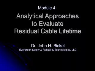
Analytical Approaches to EvaluateResidual Cable Lifetime Module 4 Dr. John H. Bickel Evergreen Safety & Reliability Technologies, LLC
Residual Cable Lifetime Assessment • Objective is to conservatively demonstrate that should design bases accident occur at end of life conditions, critical equipment will function properly • Demonstration is based on Environmental Qualification program using qualification tests performed on “pre-aged” samples.
“Pre-Aging” • Environmental Qualification programs must simulate end of life aged components • Materials are “pre-aged” before running qualification tests (simulated LOCA tests) • Elevated temperature/irradiation burn-in tests used prior to qualification tests to simulate cable conditions at end of life.
Example EQ Qualification Test Envelope for US BWR Based on Design Basis LOCA
Cable Lifetime Assessments • Two predominant failure modes are typically considered: thermal, radiation • Arrhenius thermal aging model • Radiation aging via linear dose response model. • Both need to be considered.
Arrhenius Thermal Aging Model From probability theory, mean time to failure is given by: MTTF
Arrhenius Thermal Aging Model • Probability density function is assumed to be exponential: fτ(t) = 1/ τ exp (-t/ τ ) • With time to failure given by Arrhenius law: τ = k(T)-1 = [A exp (-Φ / kT)]-1 • Mean time to failure is simply: MTTF = τ = [A exp (-Φ / kT )]-1 k = 0.8617 x 10⁻⁴ eV / °K (Boltzmann’s constant) A, Φ = experimentally derived constants
Arrhenius Thermal Aging Model • Effects of aging in elevated temperature environment can be accelerated based on: MTTF1 = [A exp (-Φ / kT1 )]-1 MTTF2 = [A exp (-Φ / kT2 )]-1 • Computing the ratio of times to failure yields:
Arrhenius Thermal Aging Model • k = 0.8617 x 10⁻⁴ eV / °K (Boltzmann’s constant) • Φis an experimentally derived constant that can be obtained from tests of specific materials • Φis more commonly assumed at low value: 0.5eV when specific material test data is not available • Lower values of Φare conservative • Unjustified use of larger Φvalues can be major source of error
Comparison of Activation Energies • Plot below shows effect of Φ= 0.5 vs. 1.0 eV
Applications of Thermal Aging Model • It is desired to qualify electrical cable that will operate in a non-radiation environment at no hotter than 40°C (313.15 °K) for a 40 year lifetime (350,400 hours). • How long should a thermal qualification test run (at different temperatures) to demonstrate cable is qualified for such environment?
Applications of Thermal Aging Model • Based on operating experience temperatures have never exceeded 30°C (303.15 °K) • After 30 years of operation, it is desired to demonstrate that cable is capable of functioning for 30 more years (e.g. 60 years – or 525,600 hours) based on lower temperatures. • Is this justifiable?
Applications of Thermal Aging Model • MTTF2 = 350,400 hours at 40°C (313.15 °K) • Solving for MTTF1 at30°C (303.15 °K) yields: • MTTF1 = 645,700 hours vs. 525,600 hours • It is justifiable.
Radiation Aging Model • Linear Dose vs. Effects is assumed • Damage = Dose (Rads) x Time (hours) • Simulate effects of 40 year plant lifetime by use of higher qualification dose rates • t1 = (D2/D1) x t2 is used for scaling
Application of Radiation Aging Model • 40 year dose to equipment ~ 4.5 x 10⁷ Rads ( or: 4.5 x 10⁵ Gy) • To run accelerated aging test to cope with radiation effects, how large a dose is required?