Download

1 / 33
330 likes | 551 Views
Comparing Two Means. Dr. Andy Field. Aims. T-tests Dependent (aka paired, matched) Independent Rationale for the tests Assumptions Interpretation Reporting results Calculating an Effect Size T -tests as a GLM. Experiments.

E N D
Comparing Two Means Dr. Andy Field
Aims • T-tests • Dependent (aka paired, matched) • Independent • Rationale for the tests • Assumptions • Interpretation • Reporting results • Calculating an Effect Size • T-tests as a GLM
Experiments • The simplest form of experiment that can be done is one with only one independent variable that is manipulated in only two ways and only one outcome is measured. • More often than not the manipulation of the independent variable involves having an experimental condition and a control. • E.g., Is the movie Scream 2 scarier than the original Scream? We could measure heart rates (which indicate anxiety) during both films and compare them. • This situation can be analysed with a t-test
T-test • Dependent t-test • Compares two means based on related data. • E.g., Data from the same people measured at different times. • Data from ‘matched’ samples. • Independent t-test • Compares two means based on independent data • E.g., data from different groups of people • Significance testing • Testing the significance of Pearson’s correlation coefficient • Testing the significance of b in regression.
Rationale to Experiments Group 1 Group 2 • Variance created by our manipulation • Removal of brain (systematic variance) • Variance created by unknown factors • E.g. Differences in ability (unsystematic variance) Lecturing Skills
Rational for the t-test • Two samples of data are collected and the sample means calculated. These means might differ by either a little or a lot. • If the samples come from the same population, then we expect their means to be roughly equal. Although it is possible for their means to differ by chance alone, we would expect large differences between sample means to occur very infrequently. • We compare the difference between the sample means that we collected to the difference between the sample means that we would expect to obtain if there were no effect (i.e. if the null hypothesis were true). We use the standard error as a gauge of the variability between sample means. If the difference between the samples we have collected is larger than what we would expect based on the standard error then we can assume one of two: • There is no effect and sample means in our population fluctuate a lot and we have, by chance, collected two samples that are atypical of the population from which they came. • The two samples come from different populations but are typical of their respective parent population. In this scenario, the difference between samples represents a genuine difference between the samples (and so the null hypothesis is incorrect). • As the observed difference between the sample means gets larger, the more confident we become that the second explanation is correct (i.e. that the null hypothesis should be rejected). If the null hypothesis is incorrect, then we gain confidence that the two sample means differ because of the different experimental manipulation imposed on each sample.
Assumptions of the t-test • Both the independent t-test and the dependent t-test are parametric tests based on the normal distribution. Therefore, they assume: • The sampling distribution is normally distributed. In the dependent t-test this means that the sampling distribution of the differences between scores should be normal, not the scores themselves. • Data are measured at least at the interval level. • The independent t-test, because it is used to test different groups of people, also assumes: • Variances in these populations are roughly equal (homogeneity of variance). • Scores in different treatment conditions are independent (because they come from different people).
Example • Is arachnophobia (fear of spiders) specific to real spiders or is a picture enough? • Participants • 12 spider phobic individuals • Manipulation • Each participant was exposed to a real spider and a picture of the same spider at two points in time. • Outcome • Anxiety
Independent vs DependentBetween Subjects vs Within Subjects For an independent or between-subjects design you need a grouping variable. For a dependent or within-subjects design (pre, post) the repeated measures for a subject are entered in rows. The first row is subject 1’s data.
Independent or Dependent? • The purpose of this experiment was to determine the differences in anxiety between real spiders and pictures of spiders. • Twelve subjects were shown a picture of a spider and a real spider. After viewing the picture or spider their anxiety was measured. The order of treatment was counterbalanced (6 shown picture first, 6 shown real spider first).
Prior to doing a dependent t-test, compute the differences and then use Explore to verify that the differences are normally distributed, see p 329. According to the K-S and S-W tests of normality the differences are normally distributed and there are no outliers.
Dependent t-test Output t(11) = 2.473, p = .031, There is a significant difference between the means, 40 ± 9.293 is significantly different from 47 ± 11.029.
Reporting the Results • On average, participants experienced significantly greater anxiety to real spiders (M = 47.00, SE = 3.18) than to pictures of spiders (M = 40.00, SE = 2.68), t(11) = −2.47, p < .05
Effect Size for Dependent t-test with G*Power 18 subjects needed to have a power of 0.80
Effect Size for Dependent t-test using Correlation Formula, p 332 r = .10 (small effect) explains 1% of the total variance. r = .30 (medium effect) explains 9% of the total variance. r = .50 (large effect) explains 25% of the total variance. In this case we would report a large effect size of .6
Example • Is arachnophobia (fear of spiders) specific to real spiders or is a picture enough? • Participants • 24 spider phobic individuals • Manipulation random assignment to: • 12 participants were exposed to a real spider • 12 were exposed to a picture of the same spider. • Outcome • Anxiety
Independent or Dependent? • The purpose of this experiment was to determine the differences in anxiety between real spiders and pictures of spiders. • 24 subjects were randomly assigned to one of the following groups: • Shown a picture of a spider • Shown a real spider. • After viewing the picture or spider their anxiety was measured.
Independent t-test Output Do the groups have equal variance? Look at Levene’s Test for Equality of Variance, Yes, p = .386, you don’t want this test to be significant. The null hypothesis is that the groups have equal variances. t(22) = −1.681, p = .107, there is no difference between the means, 40 ± 9.293 is not different from 47 ± 11.029.
Reporting the Results • On average, participants experienced greater anxiety to real spiders (M = 47.00, SE = 3.18), than to pictures of spiders (M = 40.00, SE = 2.68. This difference was not significant t(22) = −1.68, p > .05; however, it did represent a medium-sized effect r = .34.
The t-test as a GLM outcomei = (model) + errori GLM is the General Linear Model
Picture group • The group variable = 0 • Intercept = mean of baseline group
Real Spider Group • The group variable = 1 • b1= Difference between means
When Assumptions are Broken • Dependent t-test • Mann-Whitney Test • Wilcoxon rank-sum test • Independent t-test • Wilcoxon Signed-Rank Test • Robust Tests: • Bootstrapping • Trimmed means
Repeated Measures Designs are More Powerful • Ind t-test groups not diff, p = 0.107 • Dep t-test groups were different, p = 0.031 • When analyzed as though the data came from different subjects (ind t) there was no difference. • When analyzed as though the data came from the same subjects (dep t) there was a difference. • This shows that repeated measures designs are more powerful than independent (between) designs. • In a more powerful design the differences between the means will not need to be as great to find significant differences.