KINE 601 Regression & Non-parametric Statistics Reading: Huck pp 416 - 513

1. KINE 601 Regression & Non-parametric Statistics Reading: Huck pp 416 - 513

2. Regression - the statistic of prediction • Types of Regression: • bivariate (two variable) regression - also called simple linear regression • similar to Pearson correlation • one independent or predictor variable, one dependent or criterion variable • multiple regression • more than one independent variable, one dependent variable • logistic regression • using one or more independent variables to predict dichotomous classification • example: using blood pressure, cholesterol levels, and whether or not one is a diabetic to predict whether or not a person will have a heart attack within the next year (similarly, the odds ratio or relative risk of having a heart attack in the next year can be predicted) • Uses of regression: • prediction • examples: predicting GRE scores from undergraduate GPA predicting changes in HDL-C with exercise from fitness & lipid variables • explanation (which is, in fact, “backward prediction”) • example: using attitudes toward health to explain why people exercise using family & health belief information to explain why people smoke

3. Recent Use of Logistic Regression CVD Risk, Breast Cancer, and Hormone Replacement The New and Current Controversy Results from the Women’s Health Initiative - E2 + Progesterone Coronary Artery Disease Breast Cancer Stroke Pulmonary Embolism Colorectal Cancer Endometrial Cancer Hip Fracture 1.29 1.26 1.41 2.13 .63 .83 .66 JAMA, 2002, vol 288, #3 0 .5 1.0 2.0 Relative Risk (1.0 - average risk)

4. Simple Linear Regression • the regression line: Y’ = a + b (X) • Y’ is the predicted value of the dependent variable • ais a constant - represents where regression line intercepts the vertical axis • bis non-standardized regression coefficient - slope of regression line • Xis the known score or number of the independent or “predictor” variable (Y - Y’) Residuals (Error) Dependent Variable ( Y ) Regression calculates the line of best fit which minimizes the residuals b= slope (rise / run) a (intercept) Independent Variable ( X )

5. Y - Y' Y Relationshipbetween ANOVA and Regression Y Error Variance (residual) Y - Y' Y' b= slope (rise / run) Variance attributable to Regression Dependent Variable ( Y ) b Y' = a + b(X) Y Independent or “Predictor” Variable ( X ) If we made the analysis above for each data point, we could arrive at a sum of squares then a variance (mean square) for both error and the regression. This would facilitate an F - ratio that could be analyzed to test the hypothesis that b is significantly different from 0. regression MSerror MS F =

6. Example of Simple Linear Regression • A researcher wishes to determine if systolic blood pressure can be predicted using weight. Twenty subjects were recruited and were assessed for weight and systolic blood pressure. Simple linear regression analysis was performed to test the null hypothesis that no relationship exists (b = 0). Variable: SBP Sum of Mean Source DF Squares Square F Value Prob>F Model 1 4210.38190 4210.38190 54.538 0.0001 Error 18 1389.61810 77.20101 C Total 19 5600.00000 Root MSE 8.78641 R-square 0.7519 Dep Mean 140.00000 Adj R-sq 0.7381 C.V. 6.27601 Parameter Estimates Parameter Standard T for H0: Variable DF Estimate Error Parameter=0 Prob > |T| INTERCEP 1 75.754597 8.91856647 8.494 0.0001 WEIGHT 1 0.378359 0.05123363 7.385 0.0001 Standard error of the estimate -the standard deviation of the residuals. The “smaller” the SEE, the smaller the variability in the residuals and the better "fit" the regression line

7. Simple Linear Regression • Assumptions for regression: • for each value of the predictor variable, the possible true values for the corresponding observed dependent or “criterion” variable are normally distributed and have homogeneous variances. • can be checked by plotting predicted values and residuals • also a good way to spot "outliers" pattern of the residuals suggests necessary assumptions are not met the observed SBP for a given weight is random observation from the set of all normally distributed SBP's at that given weight Y (SBP) residuals outlier predicted values (Y’) from corresponding X variables X (weight)

8. Multiple Regression • the regression line:Y’ = a + b1 (X1) + b2(X2) + b3(X3)… • Y’ is the predicted value of the dependent variable • ais a constant - represents where regression line intercepts the vertical axis • bis regression coefficient - represents the mathematical contribution of the corresponding X variable to the overall regression • the sign of the b coefficients describes the nature of the relationships (direct or inverse) of the corresponding predictor variable with the criterion variable • caution: the bcoefficients must be standardized before comparisons can be made regarding the amount of variation contributed by each corresponding predictor variable. This will not be accurate however, if there is a significant relationship between any of the predictor variables • collinearity or multicollinearity • standardized regression coefficients are called beta weights and are represented by the greek letter b • X’sare the actual known score - the predictor variable values • dummy variables: coding 0's or 1's for dichotomous variables (gender) • dummy variables other than 0's or 1's are often used but should not be because the numbers (1,2,3,4,…etc.) have no quantitative meaning; ie. you cannot assume that the dependent variable changes twice as much with a dummy coded predictor variable with a X of 4 as with a dummy coded X of 2.

9. Example of Multiple Linear Regression • A researcher wishes to determine if systolic blood pressure can be predicted using weight and total cholesterol. Twenty subjects were recruited and were assessed for systolic blood pressure, weight, and total cholesterol. Multiple linear regression analysis was performed to test the null hypothesis that weight and total cholesterol have no predictive value (all b's = 0). Variable SBP Sum of Mean Source DF Squares Square F Value Prob>F Model 2 4320.70287 2160.35143 28.708 0.0001 Error 17 1279.29713 75.25277 C Total 9 5600.00000 Root MSE 8.67484 R-square 0.7716 Dep Mean 140.00000 Adj R-sq 0.7447 C.V. 6.19631 Parameter Estimates Parameter Standard T for H0: Variable DF Estimate Error Parameter=0 Prob > |T| INTERCEP 1 122.761115 39.80913557 3.084 0.0067 WEIGHT 1 0.230775 0.13197030 1.749 0.0984 TCHOL 1 -0.090914 0.07508677 -1.211 0.2425

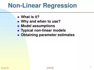
10. Types of Multiple Regression • Nonlinear Regression: Y’ = a + b1 (X1) + b2(X2)2 • also referred to as polynomial regression • used if a non-linear (curvalinear) relationship is suspected between predictor variables & the criterion variable • example: the relationship between age and maximal bench press poundage would be a parabolic (inverted “U”) relationship with an equation similar to the one above. • Stepwise Multiple Regression • variables are entered into the regression one at a time in an effort to determine which variable contributes most to the regression ("gives the most bang for the buck") • usually, the coefficient of determination(R2 ) for each equation is compared to determine if adding additional variables to the model significantly increases the capability of the model to predict the criterion variable. Other statistics such as Mallows CP may be used to determine which regression model is best.

11. Non-Parametric Statistics • Non Parametric Statistics:statistics that do not require the dependent variable to be normally distributed (there may not even be a true dependent variable) • examples of variables that are not normally distributed: • eye color, % of people who own a lawn mower, the academic rank of class members, political and moral opinions, the number of meals a person eats every year containing < 30% fat • Advantages of Non-Parametric Statistics: • no restriction of normality and variance homogeneity • computations (even by hand) are quick and speedy • Disadvantages of Non-Parametric Statistics: • less "powerful" than parametric statistics • more subjects needed to reject the null hypothesis • remember - statistics with the most power are parametric statistics when assumptions are met • since only nominal or ordinal data can be used, these methods may not fully utilize all of the information contained in the data

12. Non-Parametric Statistics • The Chi Square test - type 1: goodness of fit • tests whether or not the frequencies or proportions found in the categories of some nominal (categorical) variable fit some pre-conceived or expected pattern • are the frequencies equal? do they follow hypothesized proportions? • example: a researcher wishes to determine if the percentage of people with high blood pressure (SBP > 140) is equally distributed among a sample of Caucasians and African-Americans (normally 1 in 5 adults are hypertensive) c2= S(observed - expected)2 expected (9 - 1.8)2+ (0 - 7.2)2 + (2 - 1.8)2+ (7 - 7.2)2 1.8 7.2 1.8 7.2 = 36.03 RACE BPSTATUS Observed ‚ Expected ‚(based on 1/5 x 9 =1.8) ‚ ‚HYPER ‚NORMO ‚ Total ƒƒƒƒƒƒƒƒƒˆƒƒƒƒƒƒƒƒˆƒƒƒƒƒƒƒƒˆ AA ‚ 9 ‚ 0 ‚ 9 ‚ 1.8 ‚ 7.2 ‚ ‚ ‚ ‚ ‚ ‚ ‚ ƒƒƒƒƒƒƒƒƒˆƒƒƒƒƒƒƒƒˆƒƒƒƒƒƒƒƒˆ C ‚ 2 ‚ 7 ‚ 9 ‚ 1.8 ‚ 7.2 ‚ ‚ ‚ ‚ ‚ ‚ ‚ ƒƒƒƒƒƒƒƒƒˆƒƒƒƒƒƒƒƒˆƒƒƒƒƒƒƒƒˆ Total 11 7 18 Statistic DF Value Table Value (.05) ƒƒƒƒƒƒƒƒƒƒƒƒƒƒƒƒƒƒƒƒƒƒƒƒƒƒƒƒƒƒƒƒ Chi-Square 1 36.03 3.84 Since the calculated value exceeds the table value reject the null hypothesis that hypertension is equally distributed among Caucasians and African Americans in this sample

13. Non-Parametric Statistics • The Chi Square test - type 2: test of independence (contingence) • tests whether or not two categorical variables are independent of one another • example: a researcher wishes to determine if race and family history are independent of one another with regard to heart disease risk • H0: race (RACE) is independent of family history (FAMHIST) FAMHIST Observed ‚ Expected ‚ (row total x column total) / grand total Percent ‚ Row Pct ‚ Col Pct ‚1 ‚2 ‚3 ‚ Total ƒƒƒƒƒƒƒƒƒˆƒƒƒƒƒƒƒƒˆƒƒƒƒƒƒƒƒˆƒƒƒƒƒƒƒƒˆ AA ‚ 2 ‚ 2 ‚ 5 ‚ 9 ‚ 4 ‚ 2.5 ‚ 2.5 ‚ ‚ 11.11 ‚ 11.11 ‚ 27.78 ‚ 50.00 ‚ 22.22 ‚ 22.22 ‚ 55.56 ‚ ‚ 25.00 ‚ 40.00 ‚ 100.00 ‚ ƒƒƒƒƒƒƒƒƒˆƒƒƒƒƒƒƒƒˆƒƒƒƒƒƒƒƒˆƒƒƒƒƒƒƒƒˆ C ‚ 6 ‚ 3 ‚ 0 ‚ 9 ‚ 4 ‚ 2.5 ‚ 2.5 ‚ ‚ 33.33 ‚ 16.67 ‚ 0.00 ‚ 50.00 ‚ 66.67 ‚ 33.33 ‚ 0.00 ‚ ‚ 75.00 ‚ 60.00 ‚ 0.00 ‚ ƒƒƒƒƒƒƒƒƒˆƒƒƒƒƒƒƒƒˆƒƒƒƒƒƒƒƒˆƒƒƒƒƒƒƒƒˆ Total 8 5 5 18 44.44 27.78 27.78 100.00 Contingency Table DF Value Prob ƒƒƒƒƒƒƒƒƒƒƒƒƒƒƒƒƒƒƒƒƒƒƒƒƒƒƒƒ Chi-Square 2 7.200 0.027 Phi Coeff. .632 RACE Since p < .05 we reject the null hypothesis that race is independent of family history The special phi coefficient shows the strength of association between RACE & FAMHIST to be moderate

14. Non-Parametric Statistics tests of significance for ordinal data • Mann Whitney U - test • test for two independent samples of data that are in rank (ordinal) form • tests the medians of samples for significant differences • results in a z-score which can be compared to table values for a given level of a • non-parametric analog of an independent t - test • can be used for continuous data that are known not to be normally distributed • Wilcoxin sign rank test • test for two dependent samples of data that are in rank (ordinal) form • non-parametric analog of an dependent or correlated t - test • Kruskall-Wallace test • test for two or more independent samples that are in rank (ordinal form) • results in an H statistic that can be tested with a c2 distribution • non-parametric analog of the one way ANOVA • Friedman test • test for two or more samples in rank (ordinal) form that are correlated • results in a c2 statistic that can be tested with a c2 distribution • non-parametric analog of a one-way repeated measures ANOVA