Non-Parametric Tests
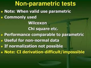
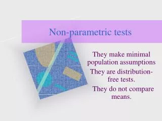
Non-Parametric Tests. Non Parametric Tests. Do not make as many assumptions about the distribution of the data as the t test. Do not require data to be Normal Good for data with outliers Non-parametric tests based on ranks of the data

Non-Parametric Tests
E N D
Presentation Transcript
Non Parametric Tests • Do not make as many assumptions about the distribution of the data as the t test. • Do not require data to be Normal • Good for data with outliers • Non-parametric tests based on ranks of the data • Work well for ordinal data (data that have a defined order, but for which averages may not make sense).
We’ll cover three non-parametric tests: *The Kruskal-Wallis Test won’t be discussed further, but explanation can be found in Rosner §12.7
Paired data example: body image Children in an orthodontia study were asked to rate how they felt about their teeth on a 5 point scale. Survey administered before and after treatment. How do you feel about your teeth? • Wish I could change them • Don’t like, but can put up with them • No particular feelings one way or the other • I am satisfied with them • Consider myself fortunate in this area
Paired data example: body image These data are • Ordinal They have a definite order, but averages may not have a clear interpretation. • Paired Two observations (before and after treatment) are made on each child. How do you feel about your teeth? • Wish I could change them • Don’t like, but can put up with them • No particular feelings one way or the other • I am satisfied with them • Consider myself fortunate in this area
Sign Test • Used for paired data • Can be ordinal or continuous • Very simple and easy to interpret • Makes no assumptions about distribution of the data • Not very powerful
Sign Test: null hypothesis • The null hypothesis for the sign test is • To evaluate H0 we only need to know the signs of the differences • If half the differences are positive and half are negative, then the median = 0 (H0 is true). • If the signs are more unbalanced, then that is evidence against H0. H0: the median difference is zero
Example: Body image data • Use the sign test to evaluate whether these data provide evidence that ortho tx improves children’s image of their teeth.
Example: Body image data • Use the sign test to evaluate whether these data provide evidence that ortho tx improves children’s image of their teeth. • First, for each child, compute the diffference between the two ratings
Example: Body image data • The sign test looks at the signs of the differences
Example: Body image data • The sign test looks at the signs of the differences • 15 children felt better about their teeth (+ difference in ratings)
Example: Body image data • The sign test looks at the signs of the differences • 15 children felt better about their teeth (+ difference in ratings) • 1 child felt worse (- diff.)
Example: Body image data • The sign test looks at the signs of the differences • 15 children felt better about their teeth (+ difference in ratings) • 1 child felt worse (- diff.) • 4 children felt the same (difference = 0)
Example: Body image data • The sign test looks at the signs of the differences • 15 children felt better about their teeth (+ difference in ratings) • 1 child felt worse (- diff.) • 4 children felt the same (difference = 0) • Looks like good evidence • Need a p-value
P-value for sign test • The p-value is the probability of an outcome as or more extreme (under H0 ) than that observed. • We observed 15 positives and 1 negative. • If H0 were true we’d expect an equal number of positive and negative differences. • More extreme outcomes would be • more than 15 positives • or less than 1 positives
P-value for sign test • P-value = P(X> 15) + P(X < 1) • X is the number of positive differences • Under H0, X is Binomial(n = 16, p = 0.5) • n = 16 because the sign test disregards the zero differences • Compute P-value using Binomial tables
Wilcoxon Signed-rank test • Wilcoxon Signed-rank test is another non-parametric test used for paired data. • It uses the magnitudes of the differences • the sign test does not • More powerful than the sign test • More difficult to interpret than the sign test
Example: Body image data • Use the Wilcoxonsigned-rank test to evaluate whether these data provide evidence that orthodontic treatment improves children’s image of their teeth.
Example: Body image data • Use the Wilcoxonsigned-rank test to evaluate whether these data provide evidence that orthodontic treatment improves children’s image of their teeth. • Work with the differences • Remove those with zero difference
Example: Body image data • To compute the test we need to
Example: Body image data • To compute the test we need to • note the signs of the differences
Example: Body image data • To compute the test we need to • note the signs of the differences • get magnitudes of the differences
Example: Body image data • To compute the test we need to • note the signs of the differences • get magnitudes of the differences • reorder the data by magnitude
Example: Body image data • To compute the test we need to • note the signs of the differences • get magnitudes of the differences • reorder the data by magnitude • assign ranks to the observations
Example: Body image data • Note that since there are many ties in the magnitudes we had to assign average ranks.
Example: Body image data For example, the 2nd through 5th differences all have the same magnitude, so we give them all the average of the 2nd through 5th rank (2+3+4+5)/4 = 3.5
Example: Body image data The statistic for the signed-rank test is the sum of the ranks of the positive differences
Example: Body image data The statistic for the signed-rank test is the sum of the ranks of the positive differences
R1: What does it mean? • With 16 observations R1 could range from 0 (all differences are negative) to 136 (all differences are positive). • If H0 were true we’d expect R1 to be near the middle of the range, in this case, 68. • R1= 132.5 appears to be evidence against H0 • Need a p-value
Signed-rank test p-value For n > 15, can use a normal approximation where ti are the numbers of ties in each group of ties (note that if ti = 1 then the term is 0), and n is the number of non-zero differences The two-sided p-value is given by
p-value for body image example There are 4 people tied with difference 2, 8 with difference 3, and 3 tied with difference 4. So And so,
p-value for signed-rank test • If n< 15 then should not use Normal approximation, but instead use an “exact” p-value. • See §13.2 in text for example of calculating an exact p-value. • In body image example, exact p-value is 0.00015.
Wilcoxon Rank Sum Test • Used to compare two independent samples • Equivalent to Mann-Whitney U test. • Like the Signed-rank test, the Rank-Sum test is based on the ranks of the data.
Example: Shear Strengths • Wish to compare two methods of preparing ceramics in terms of product strength. • Two methods of preparation • Press (n=10) • Layer (n=10) • Note outliers in “press” group • T test not appropriate • Large outliers in press group • Data likely not Normal
Computing the Wilcoxon Rank-Sum Test Statistic • Assign ranks to the combined sample • Sum the ranks in one of the groups • Which group does not matter
Computing the Wilcoxon Rank-Sum Test Statistic • Assign ranks to the combined sample • Sum the ranks in one of the groups • Which group does not matter • We’ll choose the “press” group
Computing the Wilcoxon Rank-Sum Test Statistic • Assign ranks to the combined sample • Sum the ranks in one of the groups • We’ll choose the “press” group • The “rank sum” is
Interpretation of rank sum • Like the signed-rank statistic, the rank sum does not have an obvious interpretation. • It will depend on the numbers of observations in the entire sample and in the chosen group. • In this case (total = 20, number in group = 10), R1 could range from 55 to 155. • If the groups are equal we’d expect R1to be in the middle, around 105. • R1 = 77 seems rather on the low end
Rank-sum p-value • The null hypothesis is that the two distributions are equivalent • The distribution of R1 under H0 is all possible rank sums that could occur when 10 ranks are randomly chosen from 20.
Rank-sum p-value • The p-value is the percentage of possible combinations that result in a result as extreme as R1 = 77 • 2-sided (exact) p-value is p = .0178 + .0178 = .0356 p = .0178 p = .0178
Normal approximation p-value • Exact p-value is difficult to compute. • Can use Normal approximation when both groups have at least 10 observations • See text §13.3 for computation details • In this example, the Normal approximation p-value is p=0.0376.