Download

1 / 37
400 likes | 544 Views
This comprehensive guide delves into the intricacies of RNA secondary structure modeling using context-free grammars (CFGs) and algorithms. It discusses the production rules of CFGs, illustrates how to derive sequences, and introduces key algorithms such as the Nussinov Algorithm for determining optimal structures. Readers will learn about different structural features, including hairpin loops, bulges, and multi-branched loops, while examining examples that connect theoretical concepts with real-world RNA sequences. This resource is ideal for students and researchers interested in RNA biology and computational modeling.

E N D
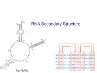
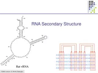
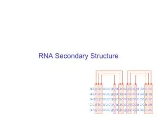
RNA Secondary Structure aagacuucggaucuggcgacaccc uacacuucggaugacaccaaagug aggucuucggcacgggcaccauuc ccaacuucggauuuugcuaccaua aagccuucggagcgggcguaacuc
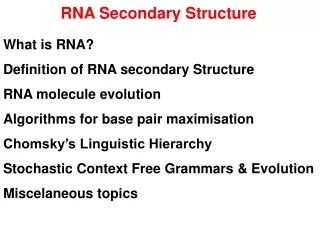
Hairpin Loops Interior loops Stems Multi-branched loop Bulge loop
Tertiary Structure Secondary Structure
A Context Free Grammar S AB Nonterminals: S, A, B A aAc | a Terminals: a, b, c, d B bBd | b Production Rules: 5 rules Derivation: • Start from the S nonterminal; • Use any production rule replacing a nonterminal with a terminal, until no more nonterminals are present S AB aAcB … aaaacccB aaaacccbBd … aaaacccbbbbbdddd Produces all strings ai+1cibj+1dj, for i, j 0
Example: modeling a stem loop AG U CG S a W1 u W1 c W2 g W2 g W3 c W3 g L c L agugc What if the stem loop can have other letters in place of the ones shown? ACGG UGCC
Example: modeling a stem loop AG U CG S a W1 u | g W1 u W1 c W2 g W2 g W3 c | g W3 u W3 g L c | a L u L agucg | agccg | cugugc More general: Any 4-long stem, 3-5-long loop: S aW1u | gW1u | gW1c | cW1g | uW1g | uW1a W1 aW2u | gW2u | gW2c | cW2g | uW2g | uW2a W2 aW3u | gW3u | gW3c | cW3g | uW3g | uW3a W3 aLu | gLu | gLc | cLg | uLg | uLa L aL1 | cL1 | gL1 | uL1 L1 aL2 | cL2 | gL2 | uL2 L2 a | c | g | u | aa | … | uu | aaa | … | uuu ACGG UGCC AG C CG GCGA UGCU CUG U CG GCGA UGUU
A parse tree: alignment of CFG to sequence AG U CG • S a W1 u • W1 c W2 g • W2 g W3 c • W3 g L c • L agucg ACGG UGCC S W1 W2 W3 L A C G G A G U G C C C G U
Alignment scores for parses! We can define each rule X s, where s is a string, to have a score. Example: W g W’ c: 3 (forms 3 hydrogen bonds) W a W’ u: 2 (forms 2 hydrogen bonds) W g W’ u: 1 (forms 1 hydrogen bond) W x W’ z -1, when (x, z) is not an a/u, g/c, g/u pair Questions: • How do we best align a CFG to a sequence? (DP) • How do we set the parameters? (Stochastic CFGs)
The Nussinov Algorithm A C C Let’s forget CFGs for a moment Problem: Find the RNA structure with the maximum (weighted) number of nested pairings A G C C G G C A U A U U A U A C A G A C A C A G U A A G C U C G C U G U G A C U G C U G A G C U G G A G G C G A G C G A U G C A U C A A U U G A ACCACGCUUAAGACACCUAGCUUGUGUCCUGGAGGUCUAUAAGUCAGACCGCGAGAGGGAAGACUCGUAUAAGCG
The Nussinov Algorithm Given sequence X = x1…xN, Define DP matrix: F(i, j) = maximum number of weighted bonds if xi…xj folds optimally Two cases, if i < j: • xi is paired with xj F(i, j) = s(xi, xj) + F(i+1, j – 1) • xi is not paired with xj F(i, j) = max{ k: i k < j } F(i, k) + F(k+1, j) i j i j i k j
The Nussinov Algorithm Initialization: F(i, i-1) = 0; for i = 2 to N F(i, i) = 0; for i = 1 to N Iteration: For l = 2 to N: For i = 1 to N – l j = i + l – 1 F(i+1, j – 1) + s(xi, xj) F(i, j) = max max{ i k < j } F(i, k) + F(k+1, j) Termination: Best structure is given by F(1, N) (Need to trace back; refer to the Durbin book)
The Nussinov Algorithm and CFGs Define the following grammar, with scores: S g S c : 3 | c S g : 3 a S u : 2 | u S a : 2 g S u : 1 | u S g : 1 S S : 0 | a S : 0 | c S : 0 | g S : 0 | u S : 0 | : 0 Note: is the “” string Then, the Nussinov algorithm finds the optimal parse of a string with this grammar
The Nussinov Algorithm Initialization: F(i, i-1) = 0; for i = 2 to N F(i, i) = 0; for i = 1 to N S a | c | g | u Iteration: For l = 2 to N: For i = 1 to N – l j = i + l – 1 F(i+1, j – 1) + s(xi, xj) S a S u | … F(i, j) = max max{ i k < j } F(i, k) + F(k+1, j) S S S Termination: Best structure is given by F(1, N)
Stochastic Context Free Grammars In an analogy to HMMs, we can assign probabilities to transitions: Given grammar X1 s11 | … | sin … Xm sm1 | … | smn Can assign probability to each rule, s.t. P(Xi si1) + … + P(Xi sin) = 1
Example S a S b : ½ a : ¼ b : ¼ Probability distribution over all strings x: x = anbn+1, then P(x) = 2-n ¼ = 2-(n+2) x = an+1bn, same Otherwise: P(x) = 0
Computational Problems • Calculate an optimal alignment of a sequence and a SCFG (DECODING) • Calculate Prob[ sequence | grammar ] (EVALUATION) • Given a set of sequences, estimate parameters of a SCFG (LEARNING)
Normal Forms for CFGs Chomsky Normal Form: X YZ X a All productions are either to 2 nonterminals, or to 1 terminal Theorem (technical) Every CFG has an equivalent one in Chomsky Normal Form (The grammar in normal form produces exactly the same set of strings)
Example of converting a CFG to C.N.F. S S ABC A Aa | a B Bb | b C CAc | c Converting: S AS’ S’ BC A AA | a B BB | b C DC’ | c C’ c D CA B C A a b c B C A A a b c a B b S S’ A B C A A a a B B D C’ b c B B C A b b c a
Another example S ABC A C | aA B bB | b C cCd | c Converting: S AS’ S’ BC A C’C’’ | c | A’A A’ a B B’B | b B’ b C C’C’’ | c C’ c C’’ CD D d
Decoding: the CYK algorithm Given x = x1....xN, and a SCFG G, Find the most likely parse of x (the most likely alignment of G to x) Dynamic programming variable: (i, j, V): likelihood of the most likely parse of xi…xj, rooted at nonterminal V Then, (1, N, S): likelihood of the most likely parse of x by the grammar
V X Y j i The CYK algorithm (Cocke-Younger-Kasami) Initialization: For i = 1 to N, any nonterminal V, (i, i, V) = log P(V xi) Iteration: For i = 1 to N – 1 For j = i+1 to N For any nonterminal V, (i, j, V) = maxXmaxYmaxik<j (i,k,X) + (k+1,j,Y) + log P(VXY) Termination: log P(x | , *) = (1, N, S) Where * is the optimal parse tree (if traced back appropriately from above)
A SCFG for predicting RNA structure S a S | c S | g S | u S | S a | S c | S g | S u a S u | c S g | g S u | u S g | g S c | u S a SS • Adjust the probability parameters to reflect bond strength etc • No distinction between non-paired bases, bulges, loops • Can modify to model these events • L: loop nonterminal • H: hairpin nonterminal • B: bulge nonterminal • etc
CYK for RNA folding Initialization: (i, i-1) = log P() Iteration: For i = 1 to N For j = i to N (i + 1, j – 1) + log P(xi S xj) (i, j – 1) + log P(S xi) (i, j) = max (i + 1, j) + log P(xi S) maxi < k < j (i, k) + (k + 1, j) + log P(S S)
Evaluation Recall HMMs: Forward: fl(i) = P(x1…xi, i = l) Backward: bk(i) = P(xi+1…xN | i = k) Then, P(x) = k fk(N) ak0 = k a0k ek(x1) bk(1) Analogue in SCFGs: Inside: a(i, j, V) = P(xi…xj is generated by nonterminal V) Outside: b(i, j, V) = P(x, excluding xi…xj is generated by S and the excluded part is rooted at V)
The Inside Algorithm To compute a(i, j, V) = P(xi…xj, produced by V) a(i, j, v) = X Y k a(i, k, X) a(k+1, j, Y) P(V XY) V X Y j i k k+1
Algorithm: Inside Initialization: For i = 1 to N, V a nonterminal, a(i, i, V) = P(V xi) Iteration: For i = 1 to N – 1 For j = i + 1 to N For V a nonterminal a(i, j, V) = X Y k a(i, k, X) a(k+1, j, X) P(V XY) Termination: P(x | ) = a(1, N, S)
The Outside Algorithm b(i, j, V) = Prob(x1…xi-1, xj+1…xN, where the “gap” is rooted at V) Given that V is the right-hand-side nonterminal of a production, b(i, j, V) = X Y k<i a(k, i – 1, X) b(k, j, Y) P(Y XV) Y V X j i k
Algorithm: Outside Initialization: b(1, N, S) = 1 For any other V, b(1, N, V) = 0 Iteration: For i = 1 to N – 1 For j = N down to i For V a nonterminal b(i, j, V) = X Y k<i a(k, i – 1, X) b(k, j, Y) P(Y XV) + X Y k<i a(j + 1, k, X) b(i, k, Y) P(Y VX) Termination: It is true for any i, that: P(x | ) = X b(i, i, X) P(X xi)
Learning for SCFGs We can now estimate c(V) = expected number of times V is used in the parse of x1….xN 1 c(V) = –––––––– 1iNijN a(i, j, V) b(i, j, V) P(x | ) 1 c(VXY) = –––––––– 1iNi<jN ik<j b(i, j, V) a(i, k, X) a(k+1, j, Y) P(VXY) P(x | )
Learning for SCFGs Then, we can re-estimate the parameters with EM, by: c(VXY) Pnew(VXY) = –––––––––––– c(V) c(V a) i: xi = a b(i, i, V) P(V a) Pnew(V a) = –––––––––– = –––––––––––––––––––––––––––––––– c(V) 1iNi<jN a(i, j, V) b(i, j, V)
Summary: SCFG and HMM algorithms GOALHMM algorithm SCFG algorithm Optimal parse Viterbi CYK Estimation Forward Inside Backward Outside Learning EM: Fw/Bck EM: Ins/Outs Memory Complexity O(N K) O(N2 K) Time Complexity O(N K2) O(N3 K3) Where K: # of states in the HMM # of nonterminals in the SCFG
position i length l 5’ 5’ position i 3’ 3’ position j position j The Zuker algorithm – main ideas Models energy of a fold in terms of specific features: • Pairs of base pairs (stacked pairs) • Bulges • Loops (size, composition) • Interactions between stem and loop position j’ positions i 5’ position j 3’