Efficient RNA Secondary Structure Prediction Using the CYK Algorithm with SCFG
440 likes | 569 Views
This document outlines the application of the CYK (Cocke-Younger-Kasami) algorithm in predicting RNA secondary structures through Stochastic Context-Free Grammars (SCFG). It details the initialization and iterative steps for dynamic programming to compute the most likely parse of RNA sequences, including probability adjustments for loops, bulges, and hairpin structures. The termination conditions and learning mechanisms, including EM (Expectation-Maximization) for SCFG parameters, are discussed alongside comparisons with HMMs (Hidden Markov Models).

Efficient RNA Secondary Structure Prediction Using the CYK Algorithm with SCFG
E N D
Presentation Transcript
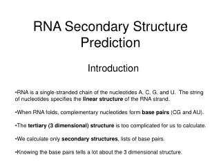
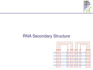
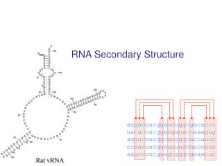
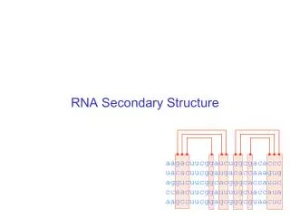
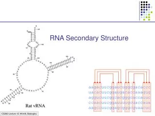
RNA Secondary Structure aagacuucggaucuggcgacaccc uacacuucggaugacaccaaagug aggucuucggcacgggcaccauuc ccaacuucggauuuugcuaccaua aagccuucggagcgggcguaacuc
Decoding: the CYK algorithm Given x = x1....xN, and a SCFG G, Find the most likely parse of x (the most likely alignment of G to x) Dynamic programming variable: (i, j, V): likelihood of the most likely parse of xi…xj, rooted at nonterminal V Then, (1, N, S): likelihood of the most likely parse of x by the grammar
V X Y j i The CYK algorithm (Cocke-Younger-Kasami) Initialization: For i = 1 to N, any nonterminal V, (i, i, V) = log P(V xi) Iteration: For i = 1 to N – 1 For j = i+1 to N For any nonterminal V, (i, j, V) = maxXmaxYmaxik<j (i,k,X) + (k+1,j,Y) + log P(VXY) Termination: log P(x | , *) = (1, N, S) Where * is the optimal parse tree (if traced back appropriately from above)
A SCFG for predicting RNA structure S a S | c S | g S | u S | S a | S c | S g | S u a S u | c S g | g S u | u S g | g S c | u S a SS • Adjust the probability parameters to reflect bond strength etc • No distinction between non-paired bases, bulges, loops • Can modify to model these events • L: loop nonterminal • H: hairpin nonterminal • B: bulge nonterminal • etc
CYK for RNA folding Initialization: (i, i-1) = log P() Iteration: For i = 1 to N For j = i to N (i+1, j–1) + log P(xi S xj) (i, j–1) + log P(S xi) (i, j) = max (i+1, j) + log P(xi S) maxi < k < j (i, k) + (k+1, j) + log P(S S)
Evaluation Recall HMMs: Forward: fl(i) = P(x1…xi, i = l) Backward: bk(i) = P(xi+1…xN | i = k) Then, P(x) = k fk(N) ak0 = l a0l el(x1) bl(1) Analogue in SCFGs: Inside: a(i, j, V) = P(xi…xj is generated by nonterminal V) Outside: b(i, j, V) = P(x, excluding xi…xj is generated by S and the excluded part is rooted at V)
The Inside Algorithm To compute a(i, j, V) = P(xi…xj, produced by V) a(i, j, v) = X Y k a(i, k, X) a(k+1, j, Y) P(V XY) V X Y j i k k+1
Algorithm: Inside Initialization: For i = 1 to N, V a nonterminal, a(i, i, V) = P(V xi) Iteration: For i = 1 to N-1 For j = i+1 to N For V a nonterminal a(i, j, V) = X Y k a(i, k, X) a(k+1, j, X) P(V XY) Termination: P(x | ) = a(1, N, S)
The Outside Algorithm b(i, j, V) = Prob(x1…xi-1, xj+1…xN, where the “gap” is rooted at V) Given that V is the right-hand-side nonterminal of a production, b(i, j, V) = X Y k<i a(k, i – 1, X) b(k, j, Y) P(Y XV) Y V X j i k
Algorithm: Outside Initialization: b(1, N, S) = 1 For any other V, b(1, N, V) = 0 Iteration: For i = 1 to N-1 For j = N down to i For V a nonterminal b(i, j, V) = X Y k<i a(k, i – 1, X) b(k, j, Y) P(Y XV) + X Y k<i a(j+1, k, X) b(i, k, Y) P(Y VX) Termination: It is true for any i, that: P(x | ) = X b(i, i, X) P(X xi)
Learning for SCFGs We can now estimate c(V) = expected number of times V is used in the parse of x1….xN 1 c(V) = –––––––– 1iNijN a(i, j, V) b(i, j, v) P(x | ) 1 c(VXY) = –––––––– 1iNi<jN ik<j b(i,j,V) a(i,k,X) a(k+1,j,Y) P(VXY) P(x | )
Learning for SCFGs Then, we can re-estimate the parameters with EM, by: c(VXY) Pnew(VXY) = –––––––––––– c(V) c(V a) i: xi = a b(i, i, V) P(V a) Pnew(V a) = –––––––––– = –––––––––––––––––––––––––––––––– c(V) 1iNi<jN a(i, j, V) b(i, j, V)
Summary: SCFG and HMM algorithms GOALHMM algorithm SCFG algorithm Optimal parse Viterbi CYK Estimation Forward Inside Backward Outside Learning EM: Fw/Bck EM: Ins/Outs Memory Complexity O(N K) O(N2 K) Time Complexity O(N K2) O(N3 K3) Where K: # of states in the HMM # of nonterminals in the SCFG
position i length l 5’ 5’ position i 3’ 3’ position j position j The Zuker algorithm – main ideas Models energy of a fold in terms of specific features: • Pairs of base pairs (stacked pairs) • Bulges • Loops (size, composition) • Interactions between stem and loop position j’ positions i 5’ position j 3’
1 4 3 5 2 5 2 3 1 4 Phylogeny Tree Reconstruction
Inferring Phylogenies Trees can be inferred by several criteria: • Morphology of the organisms • Can lead to mistakes! • Sequence comparison Example: Orc: ACAGTGACGCCCCAAACGT Elf: ACAGTGACGCTACAAACGT Dwarf: CCTGTGACGTAACAAACGA Hobbit: CCTGTGACGTAGCAAACGA Human: CCTGTGACGTAGCAAACGA
Modeling Evolution During infinitesimal time t, there is not enough time for two substitutions to happen on the same nucleotide So we can estimate P(x | y, t), for x, y {A, C, G, T} Then let P(A|A, t) …… P(A|T, t) S(t) = … … … … P(T|A, t) …… P(T|T, t) x x t y
Modeling Evolution A C Reasonable assumption: multiplicative (implying a stationary Markov process) S(t+t’) = S(t)S(t’) That is, P(x | y, t+t’) = z P(x | z, t) P(z | y, t’) Jukes-Cantor: constant rate of evolution 1 - 3 For short time , S() = I+R = 1 - 3 1 - 3 1 - 3 T G
Modeling Evolution Jukes-Cantor: For longer times, r(t) s(t) s(t) s(t) S(t) = s(t) r(t) s(t) s(t) s(t) s(t) r(t) s(t) s(t) s(t) s(t) r(t) Where we can derive: r(t) = ¼ (1 + 3 e-4t) s(t) = ¼ (1 – e-4t) S(t+) = S(t)S() = S(t)(I + R) Therefore, (S(t+) – S(t))/ = S(t) R At the limit of 0, S’(t) = S(t) R Equivalently, r’ = -3r + 3s s’ = -s + r Those diff. equations lead to: r(t) = ¼ (1 + 3 e-4t) s(t) = ¼ (1 – e-4t)
Modeling Evolution Kimura: Transitions: A/G, C/T Transversions: A/T, A/C, G/T, C/G Transitions (rate ) are much more likely than transversions (rate ) r(t)s(t)u(t)s(t) S(t) = s(t)r(t)s(t)u(t) u(t)s(t)r(t)s(t) s(t)u(t)s(t)r(t) Where s(t) = ¼ (1 – e-4t) u(t) = ¼ (1 + e-4t – e-2(+)t) r(t) = 1 – 2s(t) – u(t)
Phylogeny and sequence comparison Basic principles: • Degree of sequence difference is proportional to length of independent sequence evolution • Only use positions where alignment is pretty certain – avoid areas with (too many) gaps
Distance between two sequences Given sequences xi, xj, Define dij = distance between the two sequences One possible definition: dij = fraction f of sites u where xi[u] xj[u] Better model (Jukes-Cantor): f = 3 s(t) = ¾ (1 – e-4t) ¾ e-4t = ¾ – f log (e-4t) = log (1 – 4/3 f) -4t = log(1 – 4/3 f) dij = t = - ¼ -1 log(1 – 4/3 f)
A simple clustering method for building tree UPGMA (unweighted pair group method using arithmetic averages) Or the Average Linkage Method Given two disjoint clusters Ci, Cj of sequences, 1 dij = ––––––––– {p Ci, q Cj}dpq |Ci| |Cj| Claim that if Ck = Ci Cj, then distance to another cluster Cl is: dil |Ci| + djl |Cj| dkl = –––––––––––––– |Ci| + |Cj| Proof Ci,Cl dpq + Cj,Cl dpq dkl = –––––––––––––––– (|Ci| + |Cj|) |Cl| |Ci|/(|Ci||Cl|) Ci,Cl dpq + |Cj|/(|Cj||Cl|) Cj,Cl dpq = –––––––––––––––––––––––––––––––––––– (|Ci| + |Cj|) |Ci| dil + |Cj| djl = ––––––––––––– (|Ci| + |Cj|)
Algorithm: Average Linkage 1 4 Initialization: Assign each xi into its own cluster Ci Define one leaf per sequence, height 0 Iteration: Find two clusters Ci, Cj s.t. dij is min Let Ck = Ci Cj Define node connecting Ci, Cj, & place it at height dij/2 Delete Ci, Cj Termination: When two clusters i, j remain, place root at height dij/2 3 5 2 5 2 3 1 4
Example 4 3 2 1 v w x y z
Ultrametric Distances and Molecular Clock Definition: A distance function d(.,.) is ultrametric if for any three distances dij dik dij, it is true that dij dik = dij The Molecular Clock: The evolutionary distance between species x and y is 2 the Earth time to reach the nearest common ancestor That is, the molecular clock has constant rate in all species The molecular clock results in ultrametric distances years 1 4 2 3 5
Ultrametric Distances & Average Linkage Average Linkage is guaranteed to reconstruct correctly a binary tree with ultrametric distances Proof: Exercise 5 1 4 2 3
Weakness of Average Linkage Molecular clock: all species evolve at the same rate (Earth time) However, certain species (e.g., mouse, rat) evolve much faster Example where UPGMA messes up: AL tree Correct tree 3 2 1 3 4 4 2 1
d1,4 Additive Distances 1 Given a tree, a distance measure is additive if the distance between any pair of leaves is the sum of lengths of edges connecting them Given a tree T & additive distances dij, can uniquely reconstruct edge lengths: • Find two neighboring leaves i, j, with common parent k • Place parent node k at distance dkm = ½ (dim + djm – dij) from any node m 4 12 8 3 13 7 9 5 11 10 6 2
Reconstructing Additive Distances Given T x T D y 5 4 3 z 3 4 w 7 6 v If we know T and D, but do not know the length of each leaf, we can reconstruct those lengths
Reconstructing Additive Distances Given T x T D y z w v
Reconstructing Additive Distances Given T D x T y z a w D1 v dax = ½ (dvx + dwx – dvw) day = ½ (dvy + dwy – dvw) daz = ½ (dvz + dwz – dvw)
Reconstructing Additive Distances Given T D1 x T y 5 4 b 3 z 3 a 4 c w 7 D2 6 d(a, c) = 3 d(b, c) = d(a, b) – d(a, c) = 3 d(c, z) = d(a, z) – d(a, c) = 7 d(b, x) = d(a, x) – d(a, b) = 5 d(b, y) = d(a, y) – d(a, b) = 4 d(a, w) = d(z, w) – d(a, z) = 4 d(a, v) = d(z, v) – d(a, z) = 6 Correct!!! v D3
Neighbor-Joining • Guaranteed to produce the correct tree if distance is additive • May produce a good tree even when distance is not additive Step 1: Finding neighboring leaves Define Dij = dij – (ri + rj) Where 1 ri = –––––k dik |L| - 2 Claim: The above “magic trick” ensures that Dij is minimal iffi, j are neighbors Proof: Very technical, please read Durbin et al.! 1 3 0.1 0.1 0.1 0.4 0.4 4 2
Algorithm: Neighbor-joining Initialization: Define T to be the set of leaf nodes, one per sequence Let L = T Iteration: Pick i, j s.t. Dij is minimal Define a new node k, and set dkm = ½ (dim + djm – dij) for all m L Add k to T, with edges of lengths dik = ½ (dij + ri – rj) Remove i, j from L; Add k to L Termination: When L consists of two nodes, i, j, and the edge between them of length dij
Parsimony – What if we don’t have distances • One of the most popular methods: • GIVEN multiple alignment • FIND tree & history of substitutions explaining alignment Idea: Find the tree that explains the observed sequences with a minimal number of substitutions Two computational subproblems: • Find the parsimony cost of a given tree (easy) • Search through all tree topologies (hard)
Example {A} Final cost C = 1 {A} {A, B} Cost C+=1 A A B A {B} {A} {A} {A}
Parsimony Scoring Given a tree, and an alignment column u Label internal nodes to minimize the number of required substitutions Initialization: Set cost C = 0; k = 2N – 1 Iteration: If k is a leaf, set Rk = { xk[u] } If k is not a leaf, Let i, j be the daughter nodes; Set Rk = Ri Rj if intersection is nonempty Set Rk = Ri Rj, and C += 1, if intersection is empty Termination: Minimal cost of tree for column u, = C
Example {B} {A,B} {A} {B} {A} {A,B} {A} A A A A B B A B {A} {A} {A} {A} {B} {B} {A} {B}
Probabilistic Methods A more refined measure of evolution along a tree than parsimony P(x1, x2, xroot | t1, t2) = P(xroot) P(x1 | t1, xroot) P(x2 | t2, xroot) If we use Jukes-Cantor, for example, and x1 = xroot = A, x2 = C, t1 = t2 = 1, = pA¼(1 + 3e-4α) ¼(1 – e-4α) = (¼)3(1 + 3e-4α)(1 – e-4α) xroot t1 t2 x1 x2
Probabilistic Methods xroot • If we know all internal labels xu, P(x1, x2, …, xN, xN+1, …, x2N-1 | T, t) = P(xroot)jrootP(xj | xparent(j), tj, parent(j)) • Usually we don’t know the internal labels, therefore P(x1, x2, …, xN | T, t) = xN+1 xN+2 … x2N-1P(x1, x2, …, x2N-1 | T, t) xu x2 xN x1
Felsenstein’s Likelihood Algorithm Let P(Lk | a) denote the prob. of all the leaves below node k, given that the residue at k is a To calculate P(x1, x2, …, xN | T, t) Initialization: Set k = 2N – 1 Iteration: Compute P(Lk | a) for all a If k is a leaf node: Set P(Lk | a) = 1(a = xk) If k is not a leaf node: 1. Compute P(Li | b), P(Lj | b) for all b, for daughter nodes i, j 2. Set P(Lk | a) = b,c P(b | a, ti) P(Li | b) P(c | a, tj) P(Lj | c) Termination: Likelihood at this column = P(x1, x2, …, xN | T, t) = aP(L2N-1 | a)P(a)
Probabilistic Methods Given M (ungapped) alignment columns of N sequences, • Define likelihood of a tree: L(T, t) = P(Data | T, t) = m=1…M P(x1m, …, xnm, T, t) Maximum Likelihood Reconstruction: • Given data X = (xij), find a topology T and length vector t that maximize likelihood L(T, t)
Current popular methods HUNDREDS of programs available! http://evolution.genetics.washington.edu/phylip/software.html#methods Some recommended programs: • Discrete—Parsimony-based • Rec-1-DCM3 http://www.cs.utexas.edu/users/tandy/mp.html Tandy Warnow and colleagues • Probabilistic • SEMPHY http://www.cs.huji.ac.il/labs/compbio/semphy/ Nir Friedman and colleagues