Download

1 / 27
270 likes | 428 Views
IMR. A Regional Ice-Ocean Simulation Of the Barents and Kara Seas W. Paul Budgell Institute of Marine Research and Bjerknes Centre for Climate Research Bergen, Norway ROMS User Meeting, Venice October 18-21, 2004. IMR. Outline of Talk : Background Description of ice-ocean model

E N D
IMR A Regional Ice-Ocean Simulation Of the Barents and Kara Seas W. Paul Budgell Institute of Marine Research and Bjerknes Centre for Climate Research Bergen, Norway ROMS User Meeting, Venice October 18-21, 2004
IMR • Outline of Talk: • Background • Description of ice-ocean model • Model set-up • Simulation results • Comparison with observations
IMR • Background • Region of interest is the Barents Sea • Dynamical downscaling experiments • First replicate present-day climate • Validate with available observations
IMR Model Domain
IMR • Ocean Model Component • Community Regional Ocean Modelling • System (ROMS) version 2.1 • Terrain-following coordinate system with • generalized vertical coordinate, • curvilinear coordinates in horizontal • Wide variety of mixing schemes available • Advanced numerics, OMP and MPI parallel.
IMR • Ocean Model Component • Used 3rd-order upwind-biased horizontal advection • Used piece-wise parabolic splines in vertical, • spline vertical advection, spline Jacobian baroclinic • pressure gradient at topography • Used GLS mixing with MY2.5 parameters • No explicit horizontal viscosity or diffusivity
IMR Ice Dynamics Ice dynamics are based upon the elastic-viscous-plastic (EVP) rheology of Hunke and Dukowicz (1997), Hunke (1991) and Hunke and Dukowicz (1992). Under low deformation (rigid behaviour), the singularity is regularized by elastic waves. The response is very similar to viscous-plastic models in typical Arctic pack ice conditions. Numerical behaviour improved significantly by applying linearization of the viscosities at every EVP time step. The EVP model parallelizes very efficiently under both OpenMP And MPI.
IMR • Ice Thermodynamics • Ice thermodynamics are based upon those of Mellor and • Kantha (1989) and Häkkinen and Mellor (1992). Main features • include: • Three-level, single layer ice; single snow layer • Molecular sublayer under ice; Prandtl-type ice-ocean • boundary layer • Surface melt ponds • Forcing by short and long-wave radiation, sensible and • latent heat flux • NCEP fluxes, corrected for model surface temperature and ice • concentration, used as forcing
Model Set-up IMR
IMR • Model Set-up • Horizontal resolution of 7.8 to 10.5 km, • average of 9.3 km • 32 levels in the vertical • Flather (free surface) and Chapman • (momentum) open boundary • conditions for 2D variables • Nudging + radiation condition OBCs • for 3D-mom and tracers
IMR • Boundary and Initial Conditions • Tidal forcing from AOTIM • Coarse model used for initialization and • boundary forcing of regional model • 50 km resolution in Nordic Seas/Arctic • NCEP daily mean fluxes (Bentsen and • Drange, 2001) used for forcing • Hindcast from 1948-2002 completed, • archived 5-day mean fields
IMR Results are shown from the first year of a1990-2002 simulation SSTIce Concentration
IMR Comparison with observations: SST from PODAAC Pathfinder AVHRR best SST, ascending (day-time) orbit, 8-day, 9-km means Ice concentration from SSM/I passive micowave, daily means Bjørnøya-Fugløya CTD sections
IMR SST
IMR Sea Ice Concentration
IMR Section Locations
Ice Melt - 1993 IMR
IMR • Conclusions • Model captures seasonal variability in the Barents • Good agreement with observed ice distribution • Barents inflow is too cold, too fresh – OBC issue • Brine rejection from ice formation produces realistic water • masses • ROMS captures significant portion of mesoscale variability • even with 9-km resolution