Download
1 / 21
370 likes | 832 Views
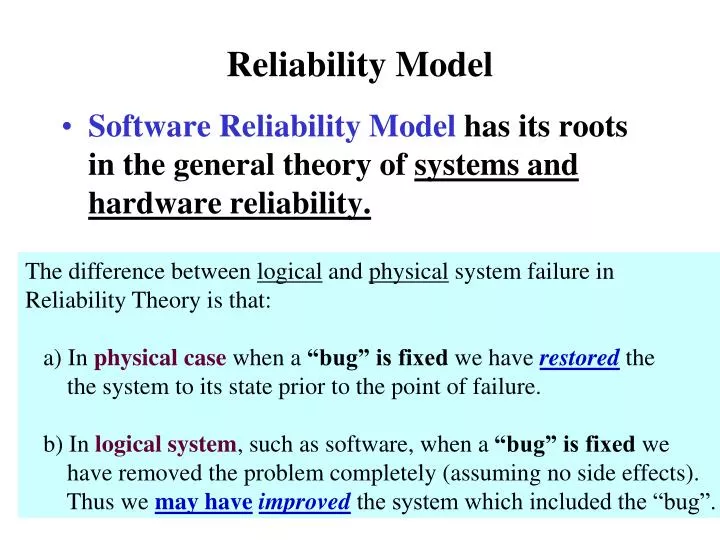
Reliability Model. Software Reliability Model has its roots in the general theory of systems and hardware reliability. The difference between logical and physical system failure in Reliability Theory is that: a) In physical case when a “bug” is fixed we have restored the

E N D
Reliability Model • Software Reliability Model has its roots in the general theory of systems and hardware reliability. The difference between logical and physical system failure in Reliability Theory is that: a) In physical case when a “bug” is fixed we have restored the the system to its state prior to the point of failure. b) In logical system, such as software, when a “bug” is fixed we have removed the problem completely (assuming no side effects). Thus we may haveimproved the system which included the “bug”.
What is Reliability ? • Previously we talked about “validity” & “reliability” of measurement/metric, saying that reliability is a measure of “consistency” ---- • Reliability of a system Z is sometimes defined as: “ theprobability that system Z runs without a failure for a specified time unit ” e.g. reliability of system Z = .99 for 100 hours = probability that Z runs without failure for 100 hours is .99 = (is this the same as saying that the system runs for 99 hours out of the 100 hours?) or = the probability of system Z fails in 100 hours is .01 (== .01bug encountered / 100 hours == 1bug encountered / 10,000 hours)
Reliability Model • Software Reliability Model is based mostly on data from the testing phase, after development is virtually complete. • The basic “goal” of Reliability Theory is to predict when the system will fail. • e.g. How can we use the existing data of time between failures {t1, t2, - - - -, tn} to predict the time to the next failure, ti , where i > n? (the data from testing provide a fairly good indication of reliability ) • The approach is based on creating a probability density function, f, of time, t, which describes when the component may fail
Sample “Creations” of Reliability Models y y time between failure # of failures y = e cx y = e –cx x x failure, x time-unit, x b) fault count model a) time between failure model
Uniform Probability Density Function Consider an “interesting” case: • A software component that has equal probability of failure within a period of x time. • That same software component will definitely not fail past the x time period.
Uniform Probability Density Function Example f(t) probability of failure f(t) = z for t between 0 and x My software ran for 1000 hours without a failure. I think I am home free, now! z f(t) = 0 for t > 0 t Time X
Uniform Probability Density Function Not very realistic for software? • For software, it is most unlikely that failure time can be bounded, such as by time x. • For software, it is also very difficultto assume that the probability of failure is uniform over the time period of [0 , x] • For software, we really do not know and thus can not bound when a failure may occur nor state that the probability of failure is equal.
Exponential Probability Density Function • Again, consider the Weibull family of distributions • f(t) = (m/t) ((t/c)m) (e**(-(t/c)m)) • Set m = 1 which will give the exponential shape • f(t) = (1/t) (t/c) (e -(t/c) ) • f(t) = (1/c) (e -(t/c) ) • This gives us the traditional Exponential probability density function or PDF • f(t) = λe -λt where λ = 1/c • The failure time is unbounded and failure occurs independently (or randomly)
exponential probability density function (PDF) for defects over time f(t) f(t) = (1/c) ( e(-t/c) ) =1/c # of problems or # of defects /kloc t time
Cumulative Distribution Function • The area under the f(t) curve is the cumulative distribution. • So F(t) = f(t) dt F(t) = 1/c (e**-(t/c)) F(t) = 1/c e**-(t/c) = (1/c)(-c) e**(-t/c) = - e –(t/c) F(t) = 1 – e (-t/c) t t 0 0
Cumulative Distribution Function(Normalized to 1 ) F(t) F(t) = 1 – e -(t/c) t
Different Ways to View the PDF and CDF • If PDF is the # of errors found at each time unit • Then the CDF is theaccumulative total # of errors found up to that time unit. (In the case of normalized CDF, it shows the % of total errors found up to that time.) • IfPDF is the probability of finding an error ateach time unit • Then the CDF is the probability of finding an error from the beginning until that time unit.
Using Reliability Model for Testing • The assumption behind time, t, needs to be considered. • What should the time unit be ? • Should it be by execution time, such as x CPU time? • For small jobs • Should it be by calendar time, such as x days or y weeks ? • For large commercial project • Is the testing homogenous at each time unit ? • Same number of test cases ran? • Same type of test cases ran? • Amount of test effort (person-hours) the same ? • If the testing effort is not homogenous, what should be done ?
One Possible Way to Normalize Non-Homogenous Testing Efforts • Accumulate all the testing hours or all the test cases and divide it by the total number of elapsed time (e.g. n weeks). Use that number as the effort-week. • Calculate the problems found (defect rate) for each of the effort-week. • Allocate the problems found for the first effort- week to the first time unit (e.g. 1st week), the problems found for the second effort-week to the second week, etc. For Example: - Total elapsed time is 12 weeks for testing. - Total testing hours is 60 person hours - then Effort-week = 60/12 = 5 person hours is 1 effort-week - then plot the problems found by effort-week (5-person-hours) of testing
How Much Data is Needed for Prediction? • Assuming that Exponential Model is the right model, then how much data is needed before one can use the function for prediction ? • There is no clear guideline • It will depend on your total time period • It will depend on how good your data is and the assumption of the homogeneity of testing • Some experiences show that at least half or more of the test has to be completed before the data could be used for projecting the remaining test period.
Reliability Models • From the basic Exponential Model, there have been numerous reliability models proposed in the literature. • Unfortunately, none has been accepted as “the” model to use for a variety of reasons: • Not tested against enough situations • Too difficult and expensive to gather enough data • Restricted to certain assumptions • Too complex for average software engineer to understand
Models for software come in same two basic flavors: • Number of faults found per unit of time • Time between failures # of Defects Found Per unit of time S-curve Weibull/Rayleigh curve Time Between failures Time Time Fault count model Time between failure model
Some Often Cited Reliability Models • Jelinski-Moranda Model assumes that failure occurs purely at random, all errors contribute equally to the cause of failure during testing, and fix time is negligible. (We will talk about this one on next slide) • Littlewood Model assumes that errors are not the same and thus contribute differently to the cause of failure during testing. • Goel-Okumoto Model assumes that test fixes make difference in that some fixes introduce more problems • Goel-Okumoto Non-homogenous Poisson Process Model assumes that the accumulative failures at time t can be modeled with a time-dependent Poisson process. • Musa-Okumoto Logarithmic Poisson Execution Time Model assumes that the fixes in the earlier test time frame has more effect than the latter ones • Yamada and et al’s S-Model assumes that there is extra time needed in failure analysis and just considering the defect detection is not enough Material on pages (211 – 216) will not be in the exam, but read to get an idea
Discussion on Jelinski-Moranda Model • Assumes that • Fix is instantaneous • Fix always works • This assumption leads to the fact that there is a “constant” improvement (decrease in rate of defect occurrence) • The failure rate function for testing at time ti between (i-1)th and ith failure is as follows: Z( ti) = Ǿ [ N – (i – 1) ] -where N is the estimated total # of defects at the beginning of test and -Ǿ is the constant increment (Ǿ ≤ 1) Z(t1) = .2[50 – (1-1)] = 10 def/day Z(t2) = .2[50 – (2-1)] = 9.8 def/day Z(t3) = .2[50 – (3-1)] = 9.6 def/day Z(t4) = .2[50 – (4-1)] = 9.4 def/day . . . gets better at a constant rate Same constant decrease Rate of Occurrence Of Failure Time units
Model Evaluation • Predictive capability of future failure based on current data. • Simplicity in concept, in data gathering needs, and in automating. • Quality of assumptions that can be met and sensible to software industry. • Applicability to a broader class of software across size, industry, performance, etc. • Capability to estimates quantities needed by a broader set of practitioners ranging from managers, analysts, testers, to designers.
Reliability Modeling Process • 1) Examine, plot, analyze, and understand the data gathered (including the time interval used, reliability, and validity) • 2) Try a few models and pick one that fits the best, understanding the underlying assumptions of the different models. • 3) Estimate the parameters used by the specific model • 4) Using the estimated parameters and decide on a specific model • 5) Use some goodness of fit analysis to compare the estimate from the model and the actual observed data. (e.g. Kolomogrov-Smirnov tests whether a specific sample is really from a particular population by examining the cumulative distribution of the sample versus that of the population.) • 6) Make the projection using the model, check against the actual data, and assess reasonableness