Download
1 / 16
170 likes | 469 Views
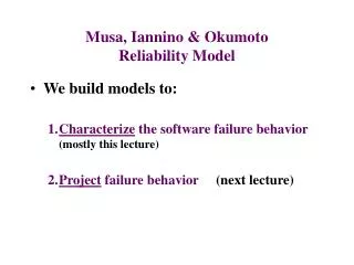
Musa, Iannino & Okumoto Reliability Model. We build models to: Characterize the software failure behavior (mostly this lecture) Project failure behavior (next lecture). Musa, Iannino & Okumoto Reliability Model. Musa-Iannino-Okumoto model(s): Covers the following models:

E N D
Musa, Iannino & OkumotoReliability Model • We build models to: • Characterize the software failure behavior (mostly this lecture) • Project failure behavior (next lecture)
Musa, Iannino & OkumotoReliability Model • Musa-Iannino-Okumoto model(s): • Covers the following models: • “failure intensity” and “# of failures experienced” • “# of failures” and “execution time” • “failure intensity” and “execution time” (next lecture notes) • Assumes failures occur as a random (non-homogeneousPoisson) process • Non-homogeneousin that, at each time point, the characteristic of the probability distribution varies ( as discussed in the previous lecture note) • Poisson is the distribution of the value of the random variable at each point in time.
A Side Note: on Poisson Distribution • Let Z be a discrete random variable that can take on values 0, 1, 2, - - - , n, --- then: P(Z = a) = [(e-δδa) / a!] , for a = 0,1, - - -,n,- - P(Z) is then said to have a Poisson distribution with the estimated parameterδ > 0, where δ is the estimated, expected value that Z would be 2 assumptions for events that display Poisson distribution: 1. the events occur with a known average rate 2. each event is independent of the last event occurrence
Poisson Distribution Curves with varying δ values • P(Z = a) = [(e -δδa) / a!] , for a = 0,1, - - -,n,- - Prob. (Z) = 1 (expected value of Z) δ δ = 4 0.3 δ = 10 0.2 0.1 Z 0.0 5 10 15
Basic Model based on (failures experienced) • The failure intensity (e.g. in # of failures percpu execution time) f(u) = f0 { 1 - (u/v) } where f0 = initial failure intensity u = (accum.) number of failures experienced v = estimated total number of failures
Basic Model(the failure intensity decrement is constant) f(u) = f0 { 1 – (u/v) } f(20) = 10 {1 – (20/100) } = 8 failure intensity is 8 failures/cpu hr after experiencing 20 failures f0=10/cpu hr failure-intensity, f u = 20 u = v =100 number of failures
Basic Model • Take the 1st derivative of the intensity function with respect to u, the number of failures, to get the rate of change: • df/du = d{f0 – f0(u/v)}/du = {d(f0)/du} - {f0/v d(u)/du} = 0 – f0/v df/du = - f0/v (this is a constant ) so we have a constant negative slope • For the previous example where f0=10 failure/cpu hr and v = 100 failures, the slope is –10/100 = -.1 or the failure-intensity decrements at a constant amount of -.1/cpu hr.
Logarithmic Poisson Model • The failure intensity based also on (failures experienced) but failure intensity decrement is variable : f(u) = f0 exp(-k u) or f0 * e-ku where f0 = initial failure intensity k = decay parameter u = number failures experienced
Logarithmic Poisson Model(failure intensity decrements non-constantly) f(u) = f0 * e -(ku) where k = .2 f(10) = 10x e(- .2 x 10) = 10 x e(-2) = 1.353 failure intensity is 1.3/cpu hr after 10 failures have been experienced f0 = 10/cpu hr failure-intensity, f u = 10 number of failures
Logarithmic Poisson Model • Take the 1st derivative of the intensity function with respect to u, the number of failures, to get the rate of change: • df/du = d{f0 e(-ku) }/du = f0 d( exp (-ku) )/du = f0 exp(-ku) d(-ku)/du = f0 exp(-ku) –k • df/du = - f0 k exp(-ku) • For the previous example where f0=10 failure/cpu hr and k =.2 , the slope is -2exp(-.2u) or the failure-intensity decrements at a variable rate, dependent on the value of u, while the relative change in intensity per failure experienced is the decay factor, k=.2
Musa – Iannino – Okumoto Failure ModelBASIC Model (based on execution time) • Number of failures after t execution time: F(t) = v { 1 – e –( f0*t/v ) } Where f0 = initial failure intensity v = estimated total number of failures t = execution time What does this curve look like ? --- as t get bigger, the e-f0*t/v approaches zero and F(t) approaches v.
An Example • Consider a software with initial failure intensity of 10/CPU hr and 100 total estimated failures. Then the estimated number of failures after time t = 20 CPU execution hours would be: F(20) = 100 { 1 – exp( - 10 * 20/100)} = 100 { 1 – exp(-2) } = 100 {1 - .135} = 100 * .865 = 86.5 or 87 failures
Musa – Iannino – Okumoto Failure ModelLogarithmic Poisson Model (based on execution time) • Number of failures after t execution time : • F(t) = 1/k * ln {( f0 * k *t) + 1} where f0 = initial failure intensity k = decay parameter t = execution time
An Example • Consider a software with initial failure intensity of 10/CPU hour and decay parameter of .05. Then the estimated number of failures after t= 15 CPU execution hours would be: F(15) = 1/.05 ln{ (10 *.05 * 15) +1} = 20 ln ( 7.5 +1) = 20 * 2.14 = 42.8 or approximately 43 failures
Total Number of Failures Expected vs Execution Time Logarithmic Poisson Model accumulative # of failures experienced Limit of v Basic Model Execution time For Logarithmic Poisson Model, the accumulative # of failures grows logarithmically; but for the Basic Model, there is an estimated V limit that the model approaches.
A Quick Comparison Initial Failure Intensity Models Other assumption Basic f0 requires estimation of V = total failures Logarithmic Poisson f0 requires estimation of K = failure intensity decay