Download
1 / 43
430 likes | 566 Views
Constructing and evaluating forward models of the terrestrial carbon cycle. Peter Thornton Terrestrial Sciences Section Climate and Global Dynamics Division NCAR. Relevance of the terrestrial carbon cycle to studies of the global climate:.

E N D
Constructing and evaluating forward models of the terrestrial carbon cycle Peter Thornton Terrestrial Sciences Section Climate and Global Dynamics Division NCAR
Relevance of the terrestrial carbon cycle to studies of the global climate: • Biophysical characteristics of the land surface depend on the interactions between surface weather, atmospheric composition and chemistry, and vegetation ecophysiology: leaf area, canopy height, Bowen ratio, relative abundance of different plant functional types. • Atmospheric concentration of CO2 depends, in part, on the dynamics of the terrestrial carbon cycle, with important variation at seasonal, interannual, decadal, and longer timescales.
Research questions: • What are the current dynamics of the terrestrial carbon cycle? • What are the likely future trends in source/sink strengths under different emission and landuse change scenarios? • How do current dynamics and likely future trends depend on coupling with climate and atmospheric chemistry? • How much model detail is required to capture the dominant spatial and temporal modes of variation in the current and likely future terrestrial carbon cycles? • How can coupled climate and carbon cycle models be evaluated?
GEP = gross ecosystem production GEP Re = total ecosystem respiration NEE = net ecosystem exchange Re MR MR = maintenance respiration GR = growth respiration HR GR HR = heterotrophic respiration NEE
Effects on NEE of natural and anthropogenic disturbances: Simulation based on recorded disturbance history at Harvard Forest NEE (gC m-2 yr-1)
Effects on NEE of anthropogenic changes in atmospheric composition and chemistry:
Terrestrial carbon cycle model evaluation over gradients in climate and disturbance history Evaluation based on observations of carbon and water budget components from seven evergreen needleleaf forest Fluxnet sites Fluxnet collaborators: B.E. Law, H.L. Gholz, K.L. Clark, E. Falge, D.S. Ellsworth, A.H. Goldstein, R.K. Monson, D. Hollinger, M. Falk, J. Chen, J.P. Sparks
Location of Fluxnet sites included in this study Base map: average annual precipitation for 1980-1997
Location of seven ENF Fluxnet sites in climate space Grey region: Complete climate space for the U.S. (lower 48) Black region: Climate space occupied by evergreen needleleaf forest in the U.S (lower 48)
Duke Forest, NC Gainesville, FL Blodgett Forest, CA Niwot Ridge, CO Wind River Crane, WA Howland Forest, ME Metolius NRA, OR
Modeling Protocol • Using the Daymet surface weather database as the model driver at all sites. • Spinup simulation to bring C and N pools into steady state: repeated 18-year record of surface weather. Using assumed levels of [CO2]atm and Ndep circa 1795 AD. • Ensemble of site history simulations, with increasing [CO2]atm (IS92a), increasing Ndep from anthropogenic sources (following Holland et al., 1997), and disturbance history as recorded at each site. All simulations ending at 2000 AD. • Evaluation of ensemble statistics at current stand age, comparison against historical observations where possible.
Daymet database of daily surface weather drivers: climate summary
Disturbance history ensembling: Each member consists of a disturbance history simulation initiated in a different year of the cyclic 18-year surface weather record.
Results: Decadal and longer timescale variations dominated by disturbance history
Results: Decadal and longer timescale variations dominated by disturbance history
Results: Relationship between NEE and GEP depends on time since disturbance, and on changing [CO2]atm and Ndep
Results: Relationship between NEE and GEP depends on time since disturbance (continued)
Results: NEE response to disturbance, changing [CO2]atm, and Ndep shows strong interaction effects
Results: NEE response to [CO2]atm for old sites near steady state depends on the rate of increase in CO2
Results: Model captures observed variability in leaf area index across the climate and disturbance history gradients
Results: Model captures observed variability in evapotranspiration across the climate and disturbance history gradients
Results: Model captures observed seasonality in evapotranspiration across the climate and disturbance history gradients
Results: Model tends to underestimate annual NEE, with strong biases at the warmest sites (FL, DU) and the old sites (ME, WR).
Results: Model in generally poor agreement with observed seasonal cycle of NEE…
Results: … but the biases are not consistently attributed to either Re or GEP.
Results: … but the biases are not consistently attributed to either Re or GEP.
Model evaluation at Metolius old-growth site: Comparison to biometric measurements of carbon budget components (all units gC m-2 yr-1)
Results: Model in generally poor agreement with observed seasonal cycle of NEE…
Results: Model agrees well with chronosequence estimates of NEE at the one site where they are available (FL)
Results: Model in generally poor agreement with observed seasonal cycle of NEE…
Re GEP MR HR GR NEE Problem: How to get rid of the double peak in seasonal cycle of NEE? Focus on the Duke Forest site…
Reducing the temperature sensitivity for MR and HR gives some improvement, but double peak persists. • Excessive reduction of temperature sensitivity for HR results in low GPP due to limited N mineralization (reduced decomposition of soil organic matter). • Have to turn to the temperature dependencies for GPP… and consider the RuBisCO enzyme.
Ribulose-1,5-bisphosphate carboxylase/oxygenase (RuBisCO) • Enzyme kinetics described by Woodrow and Berry, 1988, Ann. Rev. Plant Physiology and Plant Molecular Biology. • Enzyme activity increases exponentially with temperature (eventual irreversible decrease in activity at high temperature, as proteins denature). • RuBisCO catalyzes the fixation of CO2 (photosynthesis) and the fixation of O2 (leading to photorespiration). • The carboxylase and oxygenase reactions have different Michaelis-Menten coefficients, and these coefficients have different temperature dependencies. • These differences result in an optimal temperature for photosynthesis which does not depend directly on the temperature sensitivity for the enzyme activity.
“The values listed… are calculated from measurements of the enzyme from spinach. There may, however, be small significant differences in the kinetic properties of Rubisco from different species of C3 plants.” -Woodrow and Berry, 1988 Low Topt High Topt Re GEP GEP Re MR MR HR GR HR GR NEE NEE
Results: There is apparently a significant variation in the kinetic parameters for RuBisCO across the climate gradient.
Next steps in model parameterization and evaluation: • Find optimal kinetic parameters at each site, try to establish a dependency with simple climate indices that explains the variation in optimal temperature (underway). • Incorporate measurements from soil chambers and leaf-level gas exchange data as additional constraints. Test climate dependency of optimal temperature with these data (underway). • Expand the analysis to other plant functional types – deciduous broadleaf forest, evergreen broadleaf forest, and grasses (C3 and C4). • Bring in more extensive evaluation databases (inventory, remote sensing).
Simulated Leaf Area Index for Evergreen Needleleaf Forest, NW U.S. (Compute time approximately 70 hours running threaded code on lhotse)