Download
1 / 46
510 likes | 869 Views
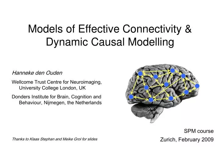
Models of Effective Connectivity & Dynamic Causal Modelling. Hanneke den Ouden Wellcome Trust Centre for Neuroimaging, University College London, UK Donders Institute for Brain, Cognition and Behaviour, Nijmegen, the Netherlands. SPM course Zurich, February 2009.

E N D
Models of Effective Connectivity & Dynamic Causal Modelling Hanneke den Ouden Wellcome Trust Centre for Neuroimaging, University College London, UK Donders Institute for Brain, Cognition and Behaviour, Nijmegen, the Netherlands SPM course Zurich, February 2009 Thanks to Klaas Stephan and Meike Grol for slides
? ? Systems analysis in functional neuroimaging Functional integration: How do regions influence each other? Brain Connectivity Functional specialisation: What regions respond to a particular experimental input?
Overview • Brain connectivity: types & definitions • anatomical connectivity • functional connectivity • effective connectivity • Functional connectivity • Psycho-physiological interactions (PPI) • Dynamic causal models (DCMs) • Applications of DCM to fMRI data
Structural, functional & effective connectivity • anatomical/structural connectivity= presence of axonal connections • functional connectivity = statistical dependencies between regional time series • effective connectivity = causal (directed) influences between neurons or neuronal populations Sporns 2007, Scholarpedia
Anatomical connectivity • presence of axonal connections • neuronal communication via synaptic contacts • visualisation by • tracing techniques • diffusion tensor imaging
However,knowing anatomical connectivity is not enough... • Connections are recruited in a context-dependent fashion: • Local functions depend on network activity
However,knowing anatomical connectivity is not enough... • Connections show plasticity • Synaptic plasticity = change in the structure and transmission properties of a synapse • Critical for learning • Can occur both rapidly and slowly • Connections are recruited in a context-dependent fashion: • Local functions depend on network activity Need to look at functional and effective connectivity
Overview • Brain connectivity: types & definitions • Functional connectivity • Psycho-physiological interactions (PPI) • Dynamic causal models (DCMs) • Applications of DCM to fMRI data
Different approaches to analysing functional connectivity Definition: statistical dependencies between regional time series • Seed voxel correlation analysis • Eigen-decomposition (PCA, SVD) • Independent component analysis (ICA) • any other technique describing statistical dependencies amongst regional time series
Seed-voxel correlation analyses • Very simple idea: • hypothesis-driven choice of a seed voxel → extract reference time series • voxel-wise correlation with time series from all other voxels in the brain seed voxel
SVCA example: Task-induced changes in functional connectivity 2 bimanual finger-tapping tasks: During task that required more bimanual coordination, SMA, PPC, M1 and PM showed increased functional connectivity (p<0.001) with left M1 No difference in SPMs! Sun et al. 2003, Neuroimage
Does functional connectivity not simply correspond to co-activation in SPMs? No, it does not - see the fictitious example on the right: Here both areas A1 and A2 are correlated identically to task T, yet they have zero correlation among themselves: r(A1,T) = r(A2,T) = 0.71 but r(A1,A2) = 0 ! regional response A1 regional response A2 task T Stephan 2004, J. Anat.
Pros & Cons of functional connectivity analyses • Pros: • useful when we have no experimental control over the system of interest and no model of what caused the data (e.g. sleep, hallucinatons, etc.) • Cons: • interpretation of resulting patterns is difficult / arbitrary • no mechanistic insight into the neural system of interest • usually suboptimal for situations where we have a priori knowledge and experimental control about the system of interest
For understanding brain function mechanistically, we need models of effective connectivity, i.e.models of causal interactions among neuronal populationsto explain regional effects in terms of interregional connectivity
Some models for computing effective connectivity from fMRI data • Structural Equation Modelling (SEM) McIntosh et al. 1991, 1994; Büchel & Friston 1997; Bullmore et al. 2000 • regression models (e.g. psycho-physiological interactions, PPIs)Friston et al. 1997 • Volterra kernels Friston & Büchel 2000 • Time series models (e.g. MAR, Granger causality)Harrison et al. 2003, Goebel et al. 2003 • Dynamic Causal Modelling (DCM)bilinear: Friston et al. 2003; nonlinear: Stephan et al. 2008
Overview • Brain connectivity: types & definitions • Functional connectivity • Psycho-physiological interactions (PPI) • Dynamic causal models (DCMs) • Applications of DCM to fMRI data
Psycho-physiological interaction (PPI) • bilinear model of how the influence of area A on area B changes by the psychological context C: A x C B • a PPI corresponds to differences in regression slopes for different contexts.
Psycho-physiological interaction (PPI) Task factor GLM of a 2x2 factorial design: Task B Task A main effect of task TA/S1 TB/S1 Stim 1 main effect of stim. type Stimulus factor interaction TB/S2 TA/S2 Stim 2 We can replace one main effect in the GLM by the time series of an area that shows this main effect. Let's replace the main effect of stimulus type by the time series of area V1: main effect of task V1 time series main effect of stim. type psycho- physiological interaction Friston et al. 1997, NeuroImage
SPM{Z} V5 activity time V1 V5 V5 attention V5 activity no attention V1 activity Example PPI: Attentional modulation of V1→V5 Attention = V1 x Att. Friston et al. 1997, NeuroImage Büchel & Friston 1997, Cereb. Cortex
V1 V5 V5 V1 PPI: interpretation Two possible interpretations of the PPI term: attention attention V1 V1 Modulation of V1V5 by attention Modulation of the impact of attention on V5 by V1
Pros & Cons of PPIs • Pros: • given a single source region, we can test for its context-dependent connectivity across the entire brain • easy to implement • Cons: • very simplistic model: only allows to model contributions from a single area • ignores time-series properties of data • operates at the level of BOLD time series sometimes very useful, but limited causal interpretability; in most cases, we need more powerful models DCM!
Overview • Brain connectivity: types & definitions • Functional connectivity • Psycho-physiological interactions (PPI) • Dynamic causal models (DCMs) • Basic idea • Neural level • Hemodynamic level • Priors & Parameter estimation • Applications of DCM to fMRI data
x λ y Basic idea of DCM for fMRI(Friston et al. 2003, NeuroImage) • Investigate functional integration & modulation of specific cortical pathways • Using a bilinear state equation, a cognitive system is modelled at its underlying neuronal level (which is not directly accessible for fMRI). • The modelled neuronal dynamics (x) is transformed into area-specific BOLD signals (y) by a hemodynamic forward model (λ). The aim of DCM is to estimate parameters at the neuronal level such that the modelled and measured BOLD signals are maximally similar.
Overview • Brain connectivity: types & definitions • Functional connectivity • Psycho-physiological interactions (PPI) • Dynamic causal models (DCMs) • Basic idea • Neural level • Hemodynamic level • Priors & Parameter estimation • Applications of DCM to fMRI data
LG left FG right LG right FG left Example: a linear system of dynamics in visual cortex LG = lingual gyrus FG = fusiform gyrus Visual input in the - left (LVF) - right (RVF)visual field. x4 x3 x1 x2 RVF LVF u1 u2
LG left FG right LG right FG left Example: a linear system of dynamics in visual cortex LG = lingual gyrus FG = fusiform gyrus Visual input in the - left (LVF) - right (RVF)visual field. x4 x3 x1 x2 RVF LVF u2 u1 systemstate input parameters state changes effective connectivity externalinputs
LG left FG right LG right FG left Extension: bilinear dynamic system x4 x3 x1 x2 CONTEXT RVF LVF u3 u2 u1
Neural state equation modulatory input u2(t) endogenous connectivity driving input u1(t) t modulation of connectivity direct inputs t y BOLD y y y λ hemodynamic model activity x2(t) activity x3(t) activity x1(t) x neuronal states integration Stephan & Friston (2007),Handbook of Brain Connectivity
Overview • Brain connectivity: types & definitions • Functional connectivity • Psycho-physiological interactions (PPI) • Dynamic causal models (DCMs) • Basic idea • Neural level • Hemodynamic level • Priors & Parameter estimation • Applications of DCM to fMRI data
t Balloon model The hemodynamic model in DCM u stimulus functions • 6 hemodynamic parameters: neural state equation important for model fitting, but of no interest for statistical inference hemodynamic state equations • Computed separately for each area (like the neural parameters) region-specific HRFs! Estimated BOLD response Friston et al. 2000, NeuroImage Stephan et al. 2007, NeuroImage
RVF LVF LG left LG right FG right FG left Example: modelled BOLD signal black: observed BOLD signal red: modelled BOLD signal
Overview • Brain connectivity: types & definitions • Functional connectivity • Psycho-physiological interactions (PPI) • Dynamic causal models (DCMs) • Basic idea • Neural level • Hemodynamic level • Priors & Parameter estimation • Applications of DCM to fMRI data
Bayesian statistics new data prior knowledge posterior likelihood ∙ prior Bayes theorem allows us to express our prior knowledge or “belief” about parameters of the model The posterior probability of the parameters given the data is an optimal combination of prior knowledge and new data, weighted by their relative precision.
Priors in DCM • embody constraints on parameter estimation • hemodynamic parameters: empirical priors • coupling parameters of self-connections: principled priors • coupling parameters other connections: shrinkage priors Small & variable effect Large & variable effect Small but clear effect Large & clear effect
DCM parameters = rate constants Integration of a first-order linear differential equation gives anexponential function: Coupling parameter is inverselyproportional to the half life of x(t): The coupling parameter athus describes the speed ofthe exponential change in x(t) If AB is 0.10 s-1 this means that, per unit time, the increase in activity in B corresponds to 10% of the activity in A
u 1 u 2 Z 1 Z 2 Example: context-dependent decay u1 stimuli u1 context u2 u2 - + - x1 x1 + x2 + x2 - - Penny, Stephan, Mechelli, Friston NeuroImage (2004)
Modulatory input (e.g. context/learning/drugs) Driving input (e.g. sensory stim) b12 c1 c2 a12 ηθ|y y BOLD y DCM Summary Select areas you want to model • Extract timeseries of these areas (x(t)) • Specify at neuronal level • what drives areas (c) • how areas interact (a) • what modulates interactions (b) • State-space model with 2 levels: • Hidden neural dynamics • Predicted BOLD response • Estimate model parameters: Gaussian a posteriori parameter distributions, characterised by mean ηθ|y and covariance Cθ|y. neuronal states activity x1(t) activity x2(t)
Inference about DCM parameters:Bayesian single-subject analysis • Gaussian assumptions about the posterior distributions of the parameters • Use of the cumulative normal distribution to test the probability that a certain parameter (or contrast of parameters cT ηθ|y) is above a chosen threshold γ: • By default, γ is chosen as zero ("does the effect exist?"). ηθ|y
Inference about DCM parameters:group analysis (classical) • In analogy to “random effects” analyses in SPM, 2nd level analyses can be applied to DCM parameters: Separate fitting of identical models for each subject Selection of bilinear parameters of interest one-sample t-test:parameter > 0 ? paired t-test:parameter 1 > parameter 2 ? rmANOVA:e.g. in case of multiple sessions per subject
Overview • Brain connectivity: types & definitions • Functional connectivity • Psycho-physiological interactions (PPI) • Dynamic causal models (DCMs) • Applications of DCM to fMRI data • Design of experiments and models • Some empirical examples and simulations
Planning a DCM-compatible study • Suitable experimental design: • any design that is suitable for a GLM • preferably multi-factorial (e.g. 2 x 2) • e.g. one factor that varies the driving (sensory) input • and one factor that varies the contextual input • Hypothesis and model: • Define specific a priori hypothesis • Which parameters are relevant to test this hypothesis? • If you want to verify that intended model is suitable to test this hypothesis, then use simulations • Define criteria for inference • What are the alternative models to test?
Task factor Stim1/ Task A Stim2/Task A Task B Task A TA/S1 TB/S1 Stim 1 GLM X1 X2 Stimulus factor Stim 2 TB/S2 TA/S2 Stim 1/ Task B Stim 2/ Task B Stim1 DCM X1 X2 Stim2 Task A Task B Multifactorial design: explaining interactions with DCM Let’s assume that an SPM analysis shows a main effect of stimulus in X1 and a stimulus task interaction in X2. How do we model this using DCM?
Simulated data A1 +++ Stim1 + Stim 1Task B Stim 2Task B Stim 2Task A Stim 1Task A A1 A2 +++ Stim2 +++ + + Task A Task B A2
X1 Stim 1Task B Stim 2Task B Stim 2Task A Stim 1Task A X2 plus added noise (SNR=1)
Final point: GLM vs. DCM DCM tries to model the same phenomena as a GLM, just in a different way: It is a model, based on connectivity and its modulation, for explaining experimentally controlled variance in local responses. If there is no evidence for an experimental effect (no activation detected by a GLM) → inclusion of this region in a DCM is not meaningful.
Thank you Stay tuned to find out how to… select the best model comparing various DCMs… test whether one region influences the connection between other regions… do DCM on your M/EEG & LFP data… and lots more!