Transferring variables between different data-sets
This presentation discusses the challenges of transferring variables between disparate datasets such as surveys and census data, often scattered across different formats. We propose a Bayesian multiple imputation (MI) approach for addressing missing data, focusing on the imputation of Left-Right self-placement scores from the SOCON 2000 dataset to the NKO 2002 dataset. This method retains variability and provides a more nuanced understanding of individual scores, ensuring broader applicability across diverse variables of interest.

Transferring variables between different data-sets
E N D
Presentation Transcript
Transferring variables between different data-sets Using imputation of individual scores Bojan Todosijevic University of Twente German Stata Users’ Meeting, April 2, 2007, Essen
The Problem: • Data scattered in different data sets – surveys, census data, etc. Typical solution: • Data aggregation – geographical, cohort. The present task: • To test a more general model for transferring data/variables between data-sets - based on the imputation of individual scores.
Advantages of the individually imputed scores: • Wider range of applications (e.g., variables of interest may be unrelated to geographic or cohort units) • Aggregation method tends to neglect variability within aggregation units; individual imputation method retains information about distribution.
The proposed approach: • A question not asked in one survey could be seen as a special case of the missing data problem (Gelman et al., 1998). • Adopt Bayesian multiple imputation (MI) (Rubin, 1987) approach. • When data are missing because a question was not asked the MAR assumption applies P(R|Ycomplete) = P(R|Yobserved)
Assessing the feasibility of the approach • Two data-sets selected - SOCON 2000 and NKO 2002 - contain a number of equivalent variables • Target variable: Left-Right self-placement – from SOCON to NKO • Test and comparisons of the ‘real’ and imputed L-R variables
Structure of the merged file type of interview | data file record | SOCON2002 NKO 2002 | Total ------------------------+----------------------+---------- NKO 2002 1st wave only | 0 333 | 333 NKO 1st and 2nd waves | 0 287 | 287 NKO 1st, 2nd and 3rd w. | 0 1,287 | 1,287 NKO 2003 only | 0 1,271 | 1,271 | | SOCON 2002 | 1,008 0 | 1,008 ------------------------+----------------------+---------- Total | 1,008 3,178 | 4,186
Imputation procedure and software ICE – MICE application for Stata (Royston, 2005) UVIS – Univariate imputation sampling • Ice imputes missing values by using switching regression, an iterative multivariable regression technique (Stata module written by Patrick Royston, 2005). The multivariate distribution is estimated from the incomplete data in a Gibbs sampling process (Van Buuren & Oudshoorn 1999). • uvis imputes missing values in the single variable based on multiple regression on a list of predictors. uvis is called repeatedly by ice in a regression switching mode to perform multivariate imputation.
Common NKO and SOCON variables Name Variable urb2 Urbanization sex Sex age Age class Class - self-description zincome Household income (standardized) educatio Education level church_a Religious service attendance party Party choice (hypothetical, vote intention, vote recollection); Employed Employment status pm Post-materialism index pol_int Political interest d_proud Proud being Dutch L-R Left-right self-placement, SOCON 2000 L-R1 Left-Right self-placement, NKO 1st wave L-R2 Left-Right self-placement, NKO 2nd wave L-R2 Left-Right self-placement, NKO 3rd wave
Imputation – three steps • 1. Imputation of the common variables in the SOCON file (using ice) • 2. Imputation of the common variables in the NKO file (using ice) • 3. Imputation of the L-R variable – from SOCON to NKO (‘the main thing’), using uvis.
Multiple Imputation - the SOCON variables Stata command for imputation: • ice l_r urb2 sex age class zincome educatio church_a party employed pm pol_int d_proud using SOCON_iced, m(5) match(l_r urb2 sex age class educatio church_a party employed pm pol_int d_proud ) cmd( urb2 class pol_int d_proud pm:regress) cycles(50) seed(14) replace
Multiple Imputation - the NKO file Stata command for imputation: • ice urb2 sex age class zincome educatio church_a party employed pm pol_int d_proud using NKO_iced, m(5)match(urb2 sex age class educatio church_a party employed pm pol_int d_proud ) cmd( urb2 class church_a pol_int d_proud pm:regress) cycles(50) seed(14) replace • L-R variables not included
Imputation of the L-R variable – from SOCON to NKO • Merged the imputed SOCON and NKO files (each containing the original and 5 imputed data-sets). • For each of the 5 imputed SOCON-NKO combinations, a univariate imputation of the L-R variable (from SOCON to NKO) was performed (using uvis). Stata command for imputation: • uvis regress l_r urb2 sex age class zincome educatio church_a party employed pm pol_int d_proud if _j==1, gen (l_r_uvis1) matchseed(14) replace Seed numbers: 1: 14, 2: 32, 3: 432, 4: 11, 5: 55.
The Imputation equation – DV: SOCON L-R Source | SS df MS Number of obs = 1008 -------------+------------------------------ F( 12, 995) = 55.22 Model | 1717.64517 12 143.137097 Prob > F = 0.0000 Residual | 2579.00563 995 2.59196546 R-squared = 0.3998 -------------+------------------------------ Adj R-squared = 0.3925 Total | 4296.65079 1007 4.26678331 Root MSE = 1.61 R = .63 ------------------------------------------------------------------------------ SOCONl_r | Coef. Std. Err. t P>|t| Beta -------------+---------------------------------------------------------------- urb2 | .0570569 .0379983 1.50 0.134 .0387282 sex | -.156749 .1075442 -1.46 0.145 -.0379609 age | -.0013591 .0043088 -0.32 0.752 -.0087341 class | .3938487 .0834685 4.72 0.000 .1461826 zincome | .0254967 .0627695 0.41 0.685 .0123456 educatio | -.1585475 .0315719 -5.02 0.000 -.1664914 church_a | -.2379957 .0522299 -4.56 0.000 -.1199417 party | .3608413 .0198037 18.22 0.000 .48643 employed | .030681 .1241836 0.25 0.805 .0068578 pm | -.2921879 .1009341 -2.89 0.004 -.0801642 pol_int | .173143 .0716642 2.42 0.016 .0685405 d_proud | -.195067 .0623608 -3.13 0.002 -.0822013 _cons | 4.659597 .5426508 8.59 0.000 . -------------+----------------------------------------------------------------
Descriptive statistics for the original and five imputed L-R variables
Correlation between the original NKO L-R variables Correlation between the imputed and original NKO L-R variables
The Imputation equation – DV: Imputed L-R R squared in 5 imputations range from Rsq=.39 to Rsq=.43. Multiple imputation parameter estimates (5 imputations) ------------------------------------------------------------------------------ l_r_Imputed | Coef. Std. Err. t P>|t| comparison with SOCON -------------+---------------------------------------------------------------- urb2 | .0750759 .0254447 2.95 0.003 became sig. sex | -.1851431 .1260133 -1.47 0.142 almost identical age | .0009682 .0037543 0.26 0.797 almost identical class | .3853003 .0718502 5.36 0.000 almost identical zincome | .0022461 .0421326 0.05 0.957 almost identical educatio | -.1453613 .0223744 -6.50 0.000 almost identical church_a | -.2166528 .0648066 -3.34 0.001 almost identical party | .3906498 .0247788 15.77 0.000 almost identical employed | .011624 .0950614 0.12 0.903 almost identical pm | -.3594543 .0790244 -4.55 0.000 increased a bit pol_int | .1972884 .101904 1.94 0.053 cf. incr., sig.dropped d_proud | -.243719 .0534851 -4.56 0.000 increased a bit _cons | 4.610467 .5392112 8.55 0.000 ------------------------------------------------------------------------------ 3178 observations (imputation 1). -------------+----------------------------------------------------------------
Comparison of the imputed with the ‘original’ NKO L-R variables
Relationships with variables NOT included in the imputation model Correction for attenuation ρimputed L-R=.40 * (1/.78)=.51
Summary of the conclusions that differ between the original and imputed variables The highest ‘missed’ correlation: with Political knowledge 1 – average for the three ‘real’ L-R variables: r=-.11.
Summary of the comparison between the imputed and original L-R variables
Summary • Coefficients associated with the imputed variables are lower in magnitude. • Correction for attenuation helps. • In a number of cases even quite low correlations were correctly predicted. • In a single case the imputed variable showed a significant relationship when the original variable showed an insignificant coefficient. • Using the imputed variable one is in danger of making Type II error, much less Type I error.
Problems to consider • Large proportion of missing values - use several ‘predictive’ data files for the imputation. • Small number of ‘predictive’ variables. • If the ‘imputationist’ and analyst are not the same person, the analyst may be interested in relationships unaccounted by the imputation model. • Imputation is done between different data sets - the major departure from the usual practice of the MI procedures.
Conclusion • The imputed variable strongly correlates with the ‘real’ responses (r is around .40, without correction for attenuation). • Multivariate model, using the variables from the prediction model, showed very close results if one used the imputed or original variables. • Univariate relationships with a broad set of attitudinal variables showed that by using imputed variable one is in danger of wrongly supporting the null-hypothesis, and underestimating the strength of the relationships. • The proposed method seems applicable especially in pilot-studies, and in studies using multiple surveys where particular questions are omitted from some studies. • Transfer of data between different sources through MI approach seems to be a reasonable alternative to aggregation.
“With our without missing data, the goal of a statistical procedure should be to make valid and efficient inferences about a population of interest – not to estimate, predict, or recover missing observations not to obtain the same results that we would have seen with complete data.” Schafer & Graham 2002, p. 149.