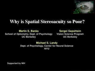
Understanding Spatial Stereoacuity Limitations: Constraints & Solutions
640 likes | 738 Views
Delve into the factors influencing poor spatial stereoacuity, from disparity precision to Nyquist frequency limits. Learn about stimulus sampling constraints, disparity gradient limits, and the correspondence problem affecting stereoacuity. Explore methodologies using random-dot stereograms for acuity assessments.

Understanding Spatial Stereoacuity Limitations: Constraints & Solutions
E N D
Presentation Transcript
Why is Spatial Stereoacuity so Poor? Martin S. Banks School of Optometry, Dept. of Psychology UC Berkeley Sergei Gepshtein Vision Science Program UC Berkeley Michael S. Landy Dept. of Psychology, Center for Neural Science NYU Supported by NIH
Depth Perception How precise is the depth map generated from disparity?
Precision of Stereopsis from Tyler (1977) • Stereo precision measured in various ways • A: Precision of detecting depth change on line of sight • D: Precision of detecting spatial variation in depth
Precision of Stereopsis from Tyler (1977) • Stereo precision measured in various ways • A: Detect depth change on line of sight • D: Precision of detecting spatial variation in depth
Precision of Stereopsis from Tyler (1977) • Stereo precision measured in various ways • A: Detect depth change on line of sight • D: Detect spatial variation in depth
Spatial Stereoacuity • Modulate disparity sinusoidally creating corrugations in depth. • Least disparity required for detection as a function of spatial frequency of corrugations: “Disparity MTF”. • Index of precision of depth map.
Disparity MTF • Disparity modulation threshold as a function of spatial frequency of corrugations. • Bradshaw & Rogers (1999). • Horizontal & vertical corrugations. • Disparity MTF: acuity = 2-3 cpd; peak at 0.3 cpd.
Luminance Contrast Sensitivity & Acuity • Luminance contrast sensitivity function (CSF): contrast for detection as function of spatial frequency. • Proven useful for characterizing limits of visual performance and for understanding optical, retinal, & post-retinal processing. • Highest detectable spatial frequency (grating acuity): 40-50 c/deg.
Disparity MTF Spatial stereoacuity more than 1 log unit lower than luminance acuity.
Disparity MTF Spatial stereoacuity more than 1 log unit lower than luminance acuity. Why is spatial stereoacuity so low?
Likely Constraints to Spatial Stereoacuity • Sampling constraints in the stimulus: Stereoacuity measured using random-element stereograms. Discrete sampling limits the highest spatial frequency one can reconstruct. • Disparity gradient limit: With increasing spatial frequency, the disparity gradient increases. If gradient approaches 1.0, binocular fusion fails. • Spatial filtering at the front end: Optical quality & retinal sampling limit acuity in other tasks, so probably limits spatial stereoacuity as well. • The correspondence problem: Manner in which binocular matching occurs presumably affects spatial stereoacuity.
Likely Constraints to Spatial Stereoacuity • Sampling constraints in the stimulus: Stereoacuity measured using random-element stereograms. Discrete sampling limits the highest spatial frequency one can reconstruct. • Disparity gradient limit: With increasing spatial frequency, the disparity gradient increases. If gradient approaches 1.0, binocular fusion fails. • Spatial filtering at the front end: Optical quality & retinal sampling limit acuity in other tasks, so probably limits spatial stereoacuity as well. • The correspondence problem: Manner in which binocular matching occurs presumably affects spatial stereoacuity.
Spatial Sampling Limit: Nyquist Frequency • Signal reconstruction from discrete samples. • At least 2 samples required per cycle. • In 1d, highest recoverable spatial frequency is Nyquist frequency: • where N is number of samples per unit distance.
Spatial Sampling Limit: Nyquist Frequency • Signal reconstruction from 2d discrete samples. • In 2d, Nyquist frequency is: • where N is number of samples in area A.
Methodology • Random-dot stereograms with sinusoidal disparity corrugations. • Corrugation orientations: +/-20 deg (near horizontal). • Observers identified orientation in 2-IFC psychophysical procedure; phase randomized. • Spatial frequency of corrugations varied according to adaptive staircase procedure. • Spatial stereoacuity threshold obtained for wide range of dot densities. • Duration = 600 msec; disparity amplitude = 16 minarc.
0.1 0.1 1 1 10 10 100 100 Spatial Stereoacuity as a function of Dot Density • Acuity proportional to dot density squared. • Scale invariance! • Asymptote at high density. 1 0.1 Spatial Stereoacuity (c/deg) 1 0.1 Dot Density (dots/deg2)
0.1 0.1 1 1 10 10 100 100 Spatial Stereoacuity & Nyquist Limit • Calculated Nyquist frequency for our displays. 1 0.1 Spatial Stereoacuity (c/deg) 1 0.1 Dot Density (dots/deg2)
0.1 0.1 1 1 10 10 100 100 Spatial Stereoacuity & Nyquist Limit Nyquist frequency • Calculated Nyquist frequency for our displays. • Acuity approx. equal to Nyquist frequency except at high densities. 1 0.1 Spatial Stereoacuity (c/deg) 1 0.1 Dot Density (dots/deg2)
Types of Random-element Stereograms Jittered-lattice: dots displaced randomly from regular lattice Sparse random: dots positioned randomly
Spatial Sampling Limit: Nyquist Frequency Same acuities with jittered-lattice and sparse random stereograms. Both follow Nyquist limit at low densities.
Likely Constraints to Spatial Stereoacuity • Sampling constraints in the stimulus: Stereoacuity measured using random-element stereograms. Discrete sampling limits the highest spatial frequency one can reconstruct. • Disparity gradient limit: With increasing spatial frequency, the disparity gradient increases. If gradient approaches 1.0, binocular fusion fails. • Spatial filtering at the front end: Optical quality & retinal sampling limit acuity in other tasks, so probably limits spatial stereoacuity as well. • The correspondence problem: Manner in which binocular matching occurs presumably affects spatial stereoacuity.
Disparity Gradient P1 P2 Disparity gradient = disparity / separation = (aR – aL) / [(aL + aR)/2] aL aR
Disparity Gradient P1 P2 P1 & P2 on horopter aR = aL, so disparity = 0 Disparity gradient = 0
Disparity Gradient P1 P1 & P2 on cyclopean line of sight aR = -aL, so separation = 0 P2 Disparity gradient =
Disparity Gradient Disparity gradient for different directions. P1 separation P2(left & right eyes) horizontal disparity
Disparity Gradient Limit • Burt & Julesz (1980): fusion as function of disparity, separation, & direction (tilt). • Set direction & horizontal disparity and found smallest fusable separation. P1 separation direction P2 (left & right eyes) disparity
Disparity Gradient Limit • Fusion breaks when disparity gradient reaches constant value. • Critical gradient = ~1. • “Disparity gradient limit”. • Limit same for all directions.
Disparity Gradient Limit • Panum’s fusion area (hatched). • Disparity gradient limit means that fusion area affected by nearby objects (A). • Forbidden zone is conical (isotropic).
Disparity Gradient & Spatial Frequency • Disparity gradient for sinusoid is indeterminant. • But for fixed amplitude, gradient proportional to spatial frequency. • We may have approached disparity gradient limit. • Tested by reducing disparity amplitude from 16 to 4.8 minarc. highest gradient peak-trough gradient Disparity (deg) Horizontal Position (deg)
0.1 0.1 1 1 10 10 100 100 Spatial Stereoacuity & Disparity Gradient Limit • Reducing disparity amplitude increases acuity at high dot densities (where DG is high). • Lowers acuity slightly at low densities (where DG is low). 1 Spatial Stereoacuity (c/deg) 0.1 1 0.1 Dot Density (dots/deg2)
Likely Constraints to Spatial Stereoacuity • Sampling constraints in the stimulus: Stereoacuity measured using random-element stereograms. Discrete sampling limits the highest spatial frequency one can reconstruct. • Disparity gradient limit: With increasing spatial frequency, the disparity gradient increases. If gradient approaches 1.0, binocular fusion fails. • Spatial filtering at the front end:Optical quality & retinal sampling limit acuity in other tasks, so probably limits spatial stereoacuity as well. • The correspondence problem: Manner in which binocular matching occurs presumably affects spatial stereoacuity.
Stereoacuity & Front-end Spatial Filtering • Low-pass spatial filtering at front-end of visual system determines high-frequency roll-off of luminance CSF. • Tested similar effects on spatial stereoacuity by: • Decreasing retinal image size of dots by increasing viewing distance. • Measuring stereoacuity as a function of retinal eccentricity. • Measuring stereoacuity as a function of blur.
Stereoacuity & Front-end Spatial Filtering • Low-pass spatial filtering at front-end of visual system determines high-frequency roll-off of luminance CSF. • Tested similar effects on spatial stereoacuity by: • Decreasing retinal image size of dots by increasing viewing distance. • Measuring stereoacuity as a function of retinal eccentricity. • Measuring stereoacuity as a function of blur.
J M A M S B 1 . 0 ) g e d / c ( y t i u c a 0 . 1 o e r e D M V T M G t S l a i t a p S 0.1 0.1 1 1 10 10 100 100 0 . 1 1 . 0 1 0 1 0 0 0 . 1 1 . 0 2 D o t D e n s i t y ( d o t / d e g ) Spatial Stereoacuity at Higher Densities N y q u i s t f r e q u e n c y • Monocular artifacts at high dot densities. • Reduce dot size to test upper limit. • Increase viewing distance from 39-154 cm. • Acuity still levels off, but at higher value. 1 M o d u l a t i o n V i e w i n g A m p l i t u d e D i s t a n c e 4 . 8 m i n 3 9 c m 4 . 8 m i n 1 5 4 c m 0.1 Spatial Stereoacuity (c/deg) 1 1 . 0 0.1 0 . 1 1 0 1 0 0 Dot Density (dots/deg2)
Stereoacuity & Front-end Spatial Filtering • Low-pass spatial filtering at front-end of visual system determines high-frequency roll-off of luminance CSF. • Tested similar effects on spatial stereoacuity by: • Decreasing retinal image size of dots by increasing viewing distance. • Measuring stereoacuity as a function of retinal eccentricity. • Measuring stereoacuity as a function of blur.
Spatial Stereoacuity & Retinal Eccentricity • Elliptical patch with sinusoidal corrugation. • Patch centered at one of three eccentricities (subject dependent). • Eccentricity random; duration = 250 ms. • Same task as before. • Again vary dot density. fixation point eccentricity 4 deg 8 deg
Spatial Stereoacuity & Retinal Eccentricity Y H H S S G T M G 1 1 . 0 Spatial Stereoacuity (c/deg) Retinal eccentricity 0 deg 0 deg 0 deg 0.1 0 . 1 6.2 5.2 6.8 12.4 10.4 13.6 1 10 100 1 10 100 0.1 1 10 100 0 . 1 1 . 0 1 0 1 0 0 1 . 0 1 0 1 0 0 1 . 0 1 0 1 0 0 Dot Density (dots/deg2) • Same acuities at low dot densities; Nyquist. • Asymptote varies significantly with retinal eccentricity.
Stereoacuity & Front-end Spatial Filtering • Low-pass spatial filtering at front-end of visual system determines high-frequency roll-off of luminance CSF. • Tested similar effects on spatial stereoacuity by: • Decreasing retinal image size of dots by increasing viewing distance. • Measuring stereoacuity as a function of retinal eccentricity. • Measuring stereoacuity as a function of blur.
Spatial Stereoacuity & Blur • We examined effect of blur on foveal spatial stereoacuity. • Three levels of blur introduced with diffusion plate: • no blur (s = 0 deg) • low blur (s = 0.12) • high blur (s = 0.25)
Spatial Stereoacuity & Blur • We examined effect of blur on foveal spatial stereoacuity. • Three levels of blur introduced with diffusion plate: • no blur (s = 0 deg) • low blur (s = 0.12) • high blur (s = 0.25)
Spatial Stereoacuity & Blur • Same acuities at low dot densities; Nyquist. • Asymptote varies significantly with spatial lowpass filtering.
Likely Constraints to Spatial Stereoacuity • Sampling constraints in the stimulus: Stereoacuity measured using random-element stereograms. Discrete sampling limits the highest spatial frequency one can reconstruct. • Disparity gradient limit: With increasing spatial frequency, the disparity gradient increases. If gradient approaches 1.0, binocular fusion fails. • Spatial filtering at the front end: Optical quality & retinal sampling limit acuity in other tasks, so probably limits spatial stereoacuity as well. • The correspondence problem:Manner in which binocular matching occurs presumably affects spatial stereoacuity.
Binocular Matching by Correlation • Binocular matching by correlation: basic and well-studied technique for obtaining depth map from binocular images. • Computer vision: Kanade & Okutomi (1994); Panton (1978) • Physiology: Ohzawa, DeAngelis, & Freeman (1990); Cumming & Parker (1997) • 2. We developed a cross-correlation algorithm for binocular matching & compared its properties to the psychophysics.
Binocular Matching by Correlation • Compute cross-correlation between eyes’ images. • Window in left eye’s image moved orthogonal to signal. • For each position in left eye, window in right eye’s image moved horizontally & cross-correlation computed. Left eye’s image Right eye’s image
Binocular Matching by Correlation • Compute cross-correlation between eyes’ images. • Window in left eye’s image moved orthogonal to signal. • For each position in left eye, window in right eye’s image moved horizontally & cross-correlation computed. Left eye’s image Right eye’s image
Binocular Matching by Correlation • Compute cross-correlation between eyes’ images. • Window in left eye’s image moved orthogonal to signal. • For each position in left eye, window in right eye’s image moved horizontally & cross-correlation computed. Left eye’s image Right eye’s image