Introduction to Spatial Interaction Models
Introduction to Spatial Interaction Models. Dr Kirk Harland and Dr Andy Evans. This Session. What is a Spatial Interaction Model? Developments in spatial interaction modelling theory. Rounding without loss or gain. Further spatial interaction model developments.

Introduction to Spatial Interaction Models
E N D
Presentation Transcript
Introduction to Spatial Interaction Models Dr Kirk Harland and Dr Andy Evans
This Session What is a Spatial Interaction Model? Developments in spatial interaction modelling theory. Rounding without loss or gain. Further spatial interaction model developments. What to use as a distance measure. Calibration.
Spatial Interaction Models • A mathematical model for simulating / predicting the interaction between two geographical features. • Interaction between features can be measured in: • goods, • information, • money, or • people
Spatial Interaction Models • A spatial interaction model has three key components: • 1) origins or origin masses, • 2) destinations or destination masses; and • 3) a representation of the relationship between each origin-destination pairs physical locations in geographical space • distance (network / Euclidean) • cost of travel • time etc…
Spatial Interaction Models • They are aggregate models and thus individuals are poorly represented. • Common applications have been: • migration (Stillwell, 1978); • journey to work (Senior, 1979); • retail location planning (Fotheringham, 1983; Fotheringham and Trew, 1993); • commercial retail marketing (Birkinet al., 2004); and • recently applied to education planning problems (Harland, 2008)
Spatial Interaction Models • The pioneering work on spatial interaction models was carried out in the 1850s. • It was based on the contemporary scientific theory of interaction between physical bodies in space, based on Sir Isaac Newton’s Theory of Universal Gravitation. • The level of interaction between two bodies varies directly proportionally to their masses and inversely with their relative locations in space.
Gravity Models • Unsurprisingly, it became known as the gravity model: • where is the predicted flow between iand j • Oiis the mass of origin zone i • Djis the mass of destination zone j • f(dij)is the distance function • k is a balancing factor or constraint ensuring flows equate to a known value
Gravity Models • Obviously, systems will have multiple origins/destinations. • These could be the same, when studying migration, for example, you may be interested in flows between wards in Leeds. • origins = Leeds wards and destination = Leeds wards • Location planning may use different features for origins and destinations. • origins = Leeds wards but the destinations could be retail outlets or schools.
Gravity Models • So an example system may look something like…
Gravity Models • But of course we need all the associated information…
Gravity Models • Once we have all the information about a system it is just a matter of iterating over all the origin-destination pairs and plugging the information into the equation…simple! • So for origin-destination pair A-X the gravity model equation would be: • k × 10 × 95.4 × f(7.499) • But what is k? • And what is f?
Gravity Models • f is a function used to represent distance decay and is usually a negative exponential. • k is simply the ratio between the simulated flow events and the observed flow events. As an equation this is: • where T is the total number of observed flow events. • For our example system this works out as:
Gravity Models • Each flow can now be calculated: • k × Oi × Dj × exp(-dij) = • (A-X) 8.57 × 10 × 95.4 × exp(-7.499) = 4.53 • (A-Y) 8.57 × 10 × 58.4 × exp(-6.979) = 4.66 • (A-Z) 8.57 × 10 × 63.9 × exp(-7.099) = 4.52 • (B-X) 8.57 × 14 × 95.4 × exp(-7.708) = 5.14 • (B-Y) 8.57 × 14 × 95.4 × exp(-7.910) = 2.57 • (B-Z) 8.57 × 14 × 95.4 × exp(-8.000) = 2.57 } The sum of all the flows = 24 (ish)
Gravity Models • The traditional way to display the result is in the form of a flow matrix, however for large datasets these can be difficult to read… Origin (i)
Issues • As noted by Wilson (1967), if we double a destination attractiveness and an origin mass the flow between the two quadruples… surely that’s not right? • The flows look fine for money but how can you have a fraction of a person moving between an origin and a destination? • Can different types of people or sectors be represented? • If we’re using zones, what do we use as a distance / cost of travel measure? • And what about calibration, how can we do that?
Developments • Wilson (1971) introduced the idea of constraints into the spatial interaction modelling theory. • The idea is to retain as much information known about a system as possible. • Through the application of constraints the issue of quadrupling interaction by doubling origin and destination masses is resolved.
Developments • Wilson’s (1971) family of spatial interaction models comprise of: • Unconstrained (or more accurately total constrained) model • Production (or origin) constrained model • Attraction (or destination) constrained model • Production-attraction (or doubly) constrained model • He also tied spatial interaction modelling to an established theory of gas particle movement and provided a sound mathematical derivation, the resulting model is known as ‘entropy maximisation’
Developments • First of all what is a constraint? • It is simply a process where some known information is incorporated into the model equation to make the numbers add up… A bit like the balancing factor but a bit more detailed • We will have a look at our example system using an origin constrained model to understand the process
Developments • An origin constrained model equation looks something like this • where • k is replaced by Ai • and Dj is replaced by W2j • It is the notation that makes the equation look complicated, it still only comprises the original terms...
Developments However, we do have to calculate the Ai balancing factor Remember that our re-ranging was: k = total real flows / simulated flow T ∑i ∑j Oi Dj exp(-1dij) However, here we want the total flows to equal only those from one origin Oi , and Oi doesn’t change on the bottom, so we can: T → Oi → 1 ∑i ∑j Oi Dj exp(-dij) ∑i ∑j Oi Dj exp(-dij) ∑j Dj exp(-dij)
Spatial Interaction Models • Subsituting W2 for D gives us: • But wait before you run out of the room this isn’t as bad as it looks… • It simply means, for each origin, sum the attractiveness estimate multiplied by the distance decay term and divide the result into 1… that’s not so bad!
Spatial Interaction Models • Using the balancing factor equation we can calculate our balancing factors by plugging in the values from our system
Spatial Interaction Models • Each flow can now be calculated using the updated equation: • Ai × Oi × Wj2 × exp(-dij) = • (A-X) 6.25 × 10 × 95.4 × exp(-7.499) = 3.30 • (A-Y) 6.25 × 10 × 58.4 × exp(-6.979) = 3.40 • (A-Z) 6.25 × 10 × 63.9 × exp(-7.099) = 3.30 • (B-X) 11.66 × 14 × 95.4 × exp(-7.708) = 7.00 • (B-Y) 11.66 × 14 × 95.4 × exp(-7.910) = 3.50 • (B-Z) 11.66 × 14 × 95.4 × exp(-8.000) = 3.50
Spatial Interaction Models Origin (i) • The new flow matrix is a much better fit than the original one. Origin (i)
Issues • As noted by Wilson (1967), if we double a destination attractiveness and an origin mass the flow between the two quadruples… surely that’s not right? • The flows look fine for money but how can you have a fraction of a person moving between an origin and a destination? • Can different types of people or sectors be represented? • If we’re using zones, what do we use as a distance / cost of travel measure? • And what about calibration, how can we do that?
Rounding without loss/gain • It is true, having fractions of persons or discrete goods flowing between areas makes no sense. • Applying conventional rounding routines can cause problems. • To exemplify this lets return to our example system, we left it like this. Origin (i)
Rounding without loss/gain • So lets just apply a conventional rounding routine to it • We have whole numbers as flows and in the destination totals • The overall total still adds up but… • The origin totals are not the same as we started with! • Using this sort of routine it is very common to end up with fewer people in the resulting matrix than we start with. Origin (i)
Rounding without loss/gain • Now let’s look at a ‘lossless’ rounding routine: • Order values in ascending order • Initialise a store variable to 0 • Add store variable to current number • Take fraction part of number and place in store variable • If not at the end of the values move to next and go to stage 3 • Place values into original order. • Because we are working towards a whole number, there shouldn’t be anything left in the store.
Rounding without loss/gain • So for origin A
Rounding without loss/gain • After applying the lossless rounding routine • We have whole numbers as flows and in the destination totals • The overall total still adds up AND • The origin totals ARE the same as we started with! • So we now have whole people or goods moving between areas Origin (i)
Rounding without loss/gain • Applying the rounding routine must be done in the same direction as the constraint application. • For origin constraints we go across the rows. • For destination constraints we go down the columns. Origin (i) Origin (i)
Issues • As noted by Wilson (1967), if we double a destination attractiveness and an origin mass the flow between the two quadruples… surely that’s not right? • The flows look fine for money but how can you have a fraction of a person moving between an origin and a destination? • Can different types of people or sectors be represented? • If we’re using zones, what do we use as a distance / cost of travel measure? • And what about calibration, how can we do that?
Developments • A great deal of effort has been put into representing different types of individuals within spatial interaction models. • One of the first methods was demonstrated by Wilson (1971). • He used different spatial interaction model configurations to represent different modes of transport in his transportation planning model. • It can be thought of as a three dimensional spatial interaction model with k being the third dimension.
Developments • Fortheringham and Trew (1993) experimented with representing different consumer choices using statistical approaches. • Other approaches have been represented in the calibration stage by using parameters specific to an origin-destination pair. • This approach has been most widely used in migration modelling (Stillwell 1978), but when applied to spatial interaction models used for planning purposes difficulties can arise if the user wants to add a destination in a scenario.
Developments • Other sector specific developments include • Incorporating elastic demand using the example of cinemas in the leisure service industry (Birkin et al., 2004). • Examining the competing and agglomeration effects of stores in the retail sector (Fotheringham, 1983). • Applying flexible capacity constraints in the education sector (Harland, 2008). • Developing a spatial interaction - agent based hybrid model for petrol price modelling (Heppenstall et al., 2005). • Although progress has been made consumers are still generally represented as groups, and this can be problematic.
Issues • As noted by Wilson (1967), if we double a destination attractiveness and an origin mass the flow between the two quadruples… surely that’s not right? • The flows look fine for money but how can you have a fraction of a person moving between an origin and a destination? • Can different types of people or sectors be represented? • If we’re using zones, what do we use as a distance / cost of travel measure? • And what about calibration, how can we do that?
Distances • This is most definitely a problem with aggregate models • We can use either network, Euclidean distances, cost of travel or time… bur where does the journey start and end? • If we are using a point as a destination then we can use the X and Y coordinate of the destination as the end point, but the origin is generally always a zone or area, so where does the journey start? • Should the closest point be used (1)? • The centroid of the zone (2)? • Maybe the furthest point (3)? 1 2 3
Distances • Perhaps the safest thing is to use the population weighted centroid… • But then what about a barrier like a river or a major road • Would the people on the right of the zone be as likely to travel to the destination shown as the those on the left 1 2 3
Distances • Using network distances can help to bring a little more realism to our model… but they also bring their own issues • Network distances are computationally intensive to calculate • Spatial interaction models require all possible origin-destination distance combinations to be calculated • For six years of school data in Leeds over 42,000,000 network distance calculations were required • If we add a destination within a ‘what if’ scenario, new network distance calculations have to be calculated ‘on the fly’
Distances • Currently, there is no one definitive answer • Assess the model utility and choose the most appropriate spatial representation • You may end up with several different spatial interaction models in a 3 dimensional layered structure similar to that of Wilson (1971), with different spatial representations in each layer
Issues • As noted by Wilson (1967), if we double a destination attractiveness and an origin mass the flow between the two quadruples… surely that’s not right? • The flows look fine for money but how can you have a fraction of a person moving between an origin and a destination? • Can different types of people or sectors be represented? • If we’re using zones, what do we use as a distance / cost of travel measure? • And what about calibration, how can we do that?
Calibration • The process of calibration is to estimate parameters in the model equation, we use parameters like β (beta) below. • where • β (beta) is a calibrated distance decay parameter • Another common parameter is the attractiveness parameter called alpha (α), which the destination attractiveness is generally raised to the power of… but we’ll just concentrate on beta today.
Calibration • By substituting different values into β we will get different resulting flow matrices. • Calibration is the process of adjusting the parameter(s) to produce the best fitting flow matrix result to observed data. • We can use different statistics such as the SRMSE or R2. • The aim is to either minimise the statistic (if the better fit between simulated and observed data is indicated by a low statistic value as with SRMSE) or maximise the statistic (if the better fit is indicated by a higher statistic value as with R2).
Calibration • Wilson (1971) used the entropy statistic to calibrate his famous entropy maximising model. • Entropy can be described as a measure of uncertainty within the resulting matrix. • By reducing entropy you reduce the uncertainty…so why did Wilson maximise it?.
Calibration • The answer is that the user / developer of a model is uncertain of the micro level events within a simulation model therefore entropy or uncertainty needs to be maximised. • But in an unconstrained model environment, this type of calibration would distribute interaction evenly across the system. • To coin an American phrase it would ‘cover all the bases’. 1 3 1 1
Calibration • The genius in the Wilson model was that he enforced constraints on the result (origin, destination and distance) to ensure that the final matrix reflected reality. • The final results maximised the uncertainty at the micro-level while enforcing macro level constraints to produce a result where all the totals added up, travelling distances were within the expected ranges and realistic interactions between zones were simulated. • Genius… but complicated, for a really good guide to the process (although the equations are quite scary) see Senior (1979).
Calibration • The spatial interaction model building process can be summarised into four stages, two of which are performed iteratively until we have a satisfactory model fit. • Planning how to calibrate and evaluate your model is crucial, and you need to think where your data is going to come from. • It is possible to over fit your model and that is why we have the evaluation stage.
Summary • Spatial interaction models are aggregate models. • They have been successfully applied in many research and commercial areas. • A few notable companies that apply variations on spatial interaction modelling theory: • ExxonMobil • Sainsbury • Tesco • Ford
Summary • Several developments in spatial interaction applications have helped to bring more realism to the spatial interaction modelling process. • The application of lossless rounding routines facilitates the modelling of individuals or discrete goods items. • However, there are still issues surrounding the selection of distance / cost of travel measures and these must be considered when developing / applying a model.
References Birkin, M., Clarke, G., Clarke, M., Culf, R. (2004). Using Spatial Models to Solve Difficult Retail Location Problems, in ‘Applied GIS and Spatial Analysis’, Eds Stillwell, J. and Clarke, G. pp. 35–54.John Wiley and Sons Ltd, Chichester Fotheringham, A. S. (1983). ‘A new set of spatial interaction models: the theory of competing destinations’. Environment and Planning A 15(1):15 – 36 Fotheringham, A. S., Trew, R. (1993). ‘Chain image and store-choice modelling: the effects of income and race’. Environment and Planning A 25:179 – 196 Harland, K. (2008).‘Journey to Learn: Geographical Mobility and Education Provision’. Unpublished PhD thesis, School of Geography, University of Leeds Heppenstall A.J., Evans A.J., Birkin M.H. (2005). A Hybrid Multi-Agent/Spatial Interaction Model System for Petrol Price Setting. Transactions in GIS. 9(1): 35 - 51. Openshaw, S. (1998). ‘Neural network, genetic, and fuzzy logic models of spatial interaction’. Environment and Planning A 30(10):1857 – 1872 Roy, J., Thill, J. C. (2004). ‘Spatial Interaction Modelling’. Papers in Regional Science 83(1):339 – 361. Senior, M. L. (1979). ‘From gravity modelling to entropy maximizing: a pedagogic guide’. Progress in Human Geography 3(2):175 – 210 Stillwell, J. C. H. (1978). ‘Interzonal migration: some historical tests of spatial-interaction models’. Environment and Planning A 10(10):1187 – 1200 Wilson, A. G. (1967). ‘A statistical theory of spatial distribution models’. Journal of Transportation Research 1:253 – 269. Wilson, A. G. (1971). ‘A family of spatial interaction models, and associated developments’. Environment and Planning 3:1 – 32