Download

1 / 95
980 likes | 1.18k Views
Operational forecasting at ECMWF: Science, Components and Products. With contributions from : Renate Hagedorn, David Richardson, Antonio Garcia Mendez, Gerald van der Grijn, Lars Isaksen and others. Ervin Zsoter ECMWF, Meteorological Operations Section ervin.zsoter@ecmwf.int. Outline.

E N D
Operational forecasting at ECMWF: Science, Components and Products With contributions from: Renate Hagedorn, David Richardson, Antonio Garcia Mendez, Gerald van der Grijn, Lars Isaksen and others Ervin Zsoter ECMWF, Meteorological Operations Section ervin.zsoter@ecmwf.int
Outline • ECMWF as an operational and research centre • EMOS – ECMWF Meteorological Observational System • Quality control at ECMWF • Important characteristics of the ECMWF’s operational analysis and forecasting system • ECMWF 4D-VAR data assimilation system • Model computational characteristics • Model performance • Some applications • Different forecast products
Czech Republic Croatia Estonia Hungary Iceland Romania Serbia and Montenegro Slovenia ECMWF as an organisation ECMWF is an independent international organization, supported by 18 member states and 8 co-operating states Convention establishing ECMWF entered into force on 1st Nov 1975 Co-operating states: Co-operating organisations:
ECMWF Budget 2006 Main Revenue 2006 Member States’contributions £27,460,600 Co-operating States’contributions £425,100 Other Revenue £1,454,600 Total£29,340,300 Main Expenditure 2006 Staff £12,961,900 Leaving Allowances& Pensions £1,807,500 ComputerExpenditure £11,785,900 Buildings £1,858,000 Supplies £927,000 Total £29,340,300
Objectives of the centre • Development of global models and data assimilation systems for the dynamics, thermodynamics and composition of the Earth’s fluid envelope and interacting parts of the Earth-system • Preparation and distribution of medium-range weather forecasts • Scientific and technical research directed towards improving the quality of these forecasts • Collection and storage of appropriate meteorological data • Make available research results and data to Member States • Provision of supercomputer resources to Member States • Assistance to WMO programmes • Advanced NWP training
Principal Goal • Maintain the current, rapid rate of improvement of its global, medium-range weather forecasting products, with particular effort on early warnings of severe weather events. • Impressive improvement in the quality of the NWP • 2-3 days over 15-20 years
Operational activities at ECMWF • Observations • Acquisition / Pre-processing / Quality control / Bias correction • Data assimilation • Dynamical fit to observations • Forecasts • Product dissemination and archiving • Verification • Operational / pre-operational validation • Data Monitoring
Data sources for the ECMWF Meteorological Operational System (EMOS) Number of observed data assimilated in 24 hours 13th February 2006
Conventional observations used BUOY: MSL Pressure, Wind-10m SYNOP/METAR/SHIP: MSL Pressure, 10m-wind, 2m-Rel.Hum. PILOT/Profilers: Wind TEMP: Land - ASAP - Dropsonde Wind, Temperature, Spec. Humidity Aircraft: Wind, Temperature
Positive trend in the number of Radiosondes reaching the upper Startosphere
Manual obs Automatic obs
28 satellite data sources used in the operational ECMWF analysis DMSP SSM/I NOAA AMSUA/B HIRS, AQUA AIRS SCATTEROMETERS GEOS TERRA / AQUA MODIS OZONE
Satellite data important • Satellite measurements are increasingly important: • Global coverage (often only source of observations over ocean and remote land) • High spatial and temporal resolution • Decrease in conventional observing networks (fewer radiosonde stations) • But satellite data are not easy to use: • Satellites do not measure the model variables (temperature, wind, humidity) • They measure radiances, so • either use derived products (e.g. cloud motion and scatterometer winds) • or calculate ‘model radiances’ and compare with observations • Recent developments in data assimilation are designed to improve the use of satellite data • Variational data assimilation: can use radiance data directly • Added model levels in upper stratosphere allow use of additional satellite data • 4D-Var: use observations at appropriate time • Increased resolution – more in agreement with resolution of measurements
Example: Tropical cyclone Bonnie near Florida satellite data complement conventional data L. Isaksen ‘Assimilation of ERS-1 and ERS-2 scatterometer winds in ERA-40’ ECMWF ERA-40 proceedings 2002
Large increase in number of observations used • Especially number of satellite data increases • A scientific and technical challenge
Observations for one 12h 4D-Var cycle 0900-2100UTC 26 March 2006 Screened Assimilated 99% of screened data is from satellites 86% of assimilated data from satellites
Observations – Quality control - Analysis Data extraction • Blacklist • Data skipped due to systematic bad performance or due to different considerations (e.g. data being assessed in passive mode) • Departures and flags available for further assessment • Check out duplicate reports • Ship tracks check • Hydrostatic check • Thinning • Skipped data to avoid Over sampling • Even so departures from FG and ANA are generated and usage flags also • 4DVAR QC • Rejections • Used data increments ANALYSIS
Observations – Quality control - Analysis • OI • 3DVAR • 4DVAR Data input Data assimilation • Raw observation • Departures (FG & AN) • Flags (data used, thinned, rejected) • Feedback files (BUFR) • ODB Monthly BUFR files for different Obs types Long term statistics
Data Monitoring (Procedures) • The basic information is included in the feedback files or ODB (feedback from the assimilation scheme) • The statistics are normally computed by comparing the observations with a FG (6 or 12 hours forecast) • Model independent statistics should be used also Co-locations • But the quality of those forecasts is not the same everywhere no fixed criteria should be applied when assessing data quality
Blacklists • The idea behind the blacklist usage is to remove from the system observations with a systematic bad performance. A blacklisted observation is considered as passive data in the data assimilation • The blacklist at ECMWF is flexible enough to consider partial blacklisting depending on • Parameters, areas, atmospheric layers, time cycles • And of course different observation types……. • MetOps Data Monitoring elaborates a proposal to update the blacklist which then is discussed with HMOS and HDA. In cases with heavy changes sensitivity experiments are carried out before implementing the new blacklist
Blacklists Quality problems in Asia & Russia
Blacklists Quality problems in Africa and southern Asia
What’s the benefit of using a blacklist? All data Ob-FG Ob-AN Used data: Blacklist and 4DVAR QC applied NH Reduced random deviation
What’s the benefit of using a blacklist? All data considered
What’s the benefit of using a blacklist? Blacklist applied
What’s the benefit of using a blacklist? Blacklist plus 4DVAR Quality Control applied
Example for data monitoring – SYNOP pressure bias correction Strong biases related to wrong station heights in the catalogue
Example for data monitoring – SYNOP pressure bias correction Bias correction applied
Pressure bias correction at ECMWF • Applied to Synop, Ship, Buoy and Metar data when needed • OI and Kalman filter schemes run in parallel • OI is used for the corrections although Kalman filtering can be switch on on request • The scheme is not applied when • The difference between the station height and the model orography is larger then 200 hPa • The observation is RDB flagged • The history of the station is not long enough
Adaptive bias correction scheme for surface pressure data • Time series of Original Ps departure, Ps bias estimate and Corrected Ps departurefor station 82353 (Dec-Apr ’05) • Once the sample size (30) was reached (Warm-up period) bias correction kicked in • Long-term bias of about -3hPa was recognised and corrected for • Station height is thought to be correct and real reason for bias is unknown • If not bias corrected the station was just surviving the “First Guess” check but to be rejected by the analysis check • When bias corrected, the station survived all the checks and was successfully used in the analysis Warm-up ≈3hPa Bias
Example for data monitoring – SYNOP pressure bias correction
Example for data monitoring – SYNOP pressure bias correction
Example for data monitoring – SYNOP pressure bias correction
ECMWF’s operational analysis and forecasting system The comprehensive earth-system model developed at ECMWF forms the basis for all the data assimilation and forecasting activities. All the main applications required are available through one integrated computer software system (a set of computer programs written in Fortran) called the Integrated Forecast System or IFS • Numerical scheme • Spectral model - TL799L91 (799 waves around a great circle on the globe, 91 hybrid vertical levels 0-80 km (0.01 hPa)) • Semi-Lagrangian time scheme • 12 minutes timestep • Prognostic variables: • wind, temperature, humidity, cloud fraction and water/ice content, pressure at surface grid-points, ozone • Grid: • Gaussian grid for physical processes, ~25 km, 76,757,590 grid points (843,490 on the surface)
Spectral and grid point representations • ECMWF model uses both spectral and grid point representations • Most upper air model variables (wind, temperature) are stored as spectral fields • Horizontal derivatives of these variables are calculated in spectral space • Surface variables and upper air humidity are stored in grid point space • Dynamical tendencies and physical parameterizations are calculated in grid point space • Resolution is the same in physical (grid point) and spectral space • Grid: • Gaussian grid for physical processes, ~25 km, 76,757,590 grid points (843,490 / level) • ‘Gaussian grid’ is regular in latitude, almost regular in longitude • On regular grid (same number of points on each latitude row) points get closer together nearer the poles • ‘Reduced Gaussian grid’ keeps distance between points nearly constant over globe
Model approximations: orography and spatial resolution High spatial resolution is needed to impose accurate boundary conditions. For example, the representation of the orography becomes more realistic with increased horizontal resolution. T255 orography, grid spacing ~80 km T799 orography, grid spacing ~25 km
Katrina (2005 Aug): 90h forecasts - T511 versus T799 Central pressure 909hPa, 785mm/24h rain T799 Central pressure 940hPa, 448mm/24h rain T511
Hurricane Gordon – T799 forecast AN 30 hrs 78 hrs 126 hrs
Grid box 25 km x 25 km Limitation: Model grid box still large
Data assimilation for weather prediction The FORECAST is computed on a grid over the globe. The meteorological OBSERVATIONS can be taken at any location in the grid. The computer model’s prediction of the atmosphere is compared against the available observations, in near real time A short-range forecast provides an estimate of the atmosphere that is compared with the observations. The two kinds of information are combined to form a corrected atmospheric state: the analysis. Corrections are computed and applied twice per day. This process is called ‘Data Assimilation’.
4D-Var Data assimilation Analysis Background values = Analysis values = Observations= 12-hourforecast Model variables, e.g. temperature “True” state of the atmosphere 12 UTC 13 March 00 UTC 13 March 00 UTC 14 March 12 UTC 14 March Time
A few 4D-Var Characteristics All observations within a 12-hour period (~3,300,000) are used simultaneously in one global (iterative) estimation problem • Observation minus model differences are computed at the observation time using the full forecast model at T799 (25 km) resolution • 4D-Var finds the 12-hour forecast evolution that optimally fits the available observations. A linearized forecast model is used in the minimization process based on the adjoint method (2 minimisation loops – T95/T255) • It does so by adjusting surface pressure, the upper-air fields of temperature, wind, specifichumidity and ozone • The analysis vector consists of 30,000,000 elements at T255 resolution (80 km) 9z 12z 15z 18z 21z
ECMWF 4D-Var procedure Use all data in a 12-hour window (0900-2100 UTC for 1200 UTC analysis) • Group observations into ½ hour time slots • Run the T799 (25km) high resolution forecast from the previous analysis and compute “observation”- “model” differences • Adjust the model fields at the start of assimilation window (0900 UTC) so the 12-hour forecast better fits the observations. This is an iterative process using a lower resolution linearized model T255 (80 km) and its adjoint model • Rerun the T799 high resolution model from the modified (improved) initial state and calculate new observation departures • The 3-4 loop in repeated twice to produce a good high resolution estimate of the atmospheric state – the result is the ECMWF analysis
Multi-incremental quadratic 4D-Var at ECMWF T799L91 T95L91 T255L91