Download
1 / 59
610 likes | 845 Views
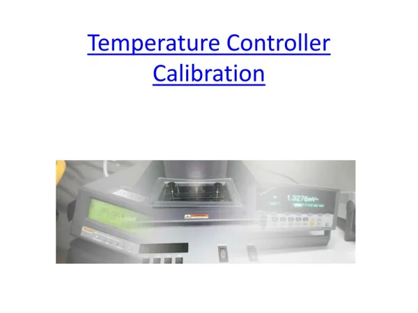
Chapter 9 Calibration of Temperature Sensors. I recommended also the calibration of the couples in term of the fixed points of boding or fusion of certain pure substances Henri LeClwtelier (1885). 9.1 GENERAL REMARKS

E N D
I recommended also the calibration of the couples in term of the fixed points of boding or fusion of certain pure substances Henri LeClwtelier (1885)
9.1 GENERAL REMARKS As seen in Chapter 4, temperature is defined by certain standards. We want to transfer this information to some more rugged, faster, cheaper, smaller device that is also temperature sensitive, and that may be carried from the standards Laboratory to a job site. Calibration consists of determining the indication or output of a temperature sensor with respect to that of a standard at a sufficient number of known temperatures so that, with acceptable means of interpolation, the indication or output of the sensor will be known over the entire temperature range of use [ 1].
Calibration problem areas are immediately apparent. There must be available: (1)a means for measuring the output of the temperature sensor, (2) a satisfactory temperature standard, (3) controlled temperature environments, and (4) a scheme for interpolating between calibration points. As a result of proper attention to application details, the means for measuring indications or outputs of all common temperature sensors within acceptable uncertainties are available (see, for example, Chapters 5-7).
A practical, realizable temperature standard has been described in the text of the IPTS (see Chapter 4) wherein temperature is defined by certain fixed points, certain standard instruments and certain standard interpolating equations. The availability and use of controlled-temperature environments wherein sensor outputs are determined, and the bases of several schemes that are useful for interpolating between the calibration points are discussed in the next sections.
9.2 CONTROLLED TEMPERATURE ENVIRONMENTS Calibration environments can be divided into two classes depending on the method of determining the temperature of die test sensor. In one case,the sensor is exposed to a fixed-paint environment that, under certain prescribed conditions , naturally exhibits a state of quasi-thermal equilibrium whose temperature is established numerically by the 1PTS without recourse to a temperature standard. In the other case, the sensor and a temperature standard are expose simultaneously controlled-temperature environment whose temperature established by the standard instrument.
Fixed-Point Baths • Three general types of fixed-point baths are commercially available. • These are the liquid-solid (freezing-point), the liquid-vapor (boiling-point), and the solid-liquid-vapor (triple-point) baths. In these fixed-point baths, use is made of the reproducible temperature-time plateau that exists and signifies the coexistence of two more phases of a substance. • Provided the sensor is not contaminated by the fixed-point material, that sufficient immersion exists, that the fixed-point sample is pure and at a uniform temperature, the temperature assigned to the bath (and hence to the sensor) is reliable.
9.2.2 Triple Point of water Of the triple-point baths, only that of water is of general interest. This bath provides the primary defining point on IPTS-68, and has been described is great detail in the various texts defining the IPTS (see Chapter 4). A pressure temperature diagram, is give in Figure 9.1a and indicates that three phase of water can coexist only at a pressure of 4.58 mm Hg. A cross-sector diagram of the cell is given in Figure 9.1b. Essentially, the cell consists of glass cylinder that has beets evacuated at the required low pressure, charged very high-purity gas-free water, and hermetically sealed.
The construction and preparation of the triple point cell are described in literature [2]-[7]. The following is a brief review. The cell is first chilled it ice path. The reentrant tube of the cell serves several purposes. It is used in thermometer well. and it is used to set up the triple point. Freezing of a port of the scaled-in water is accomplished by pouring powdered dry ice (i.e. C into the recent rant tube. When the mantle of ice, fluxes around the recent thermometer well, reaches a thickness of about 5 mm, the dry ice is removed。
The cell is again placed in an ice bath. A rod, initially at room temperature, is inserting in the reentrant well, and this melts some of the ice mantle that a thin layer of very pure water forms adjacent to the well wall. When the ice mantle is free from the reentrant tube, the triple point is established. To assure good thermal contact between the three-phase water and the thermometer. the well is filled with alcohol or mineral oil. It has been reported [6] that a properly aged ice mantle may be kept for several months with no appreciable drift in the triple-point temperature.
Several triple-point baths are commercially available. But such baths are not normally used as routine calibration environment because of tee time and care required in their preparation and use. For standards work they are, of course, a necessity.
9.2.3 Freezing Point of Water The importance of the freezing point of water (ice bath) cannot be over-emphasized. The ice bath is used extensively as the reference junction environment for most thermocouple systems, and as a calibration reference temperature for all other temperature-sensing systems. The thermocouple reference junction must be maintained at a constant and known temperature, and this temperature must be stated as a necessary part of the calibration results.
Caldwell [10] presents useful curves effects of wire site, thermal conduction, and immersion depths on the reference junction temperatures of various chromel-alumel thermocouples in ice baths. He indicates that the most potent variable is the size of the copper wire used to connect the reference junctions to the measuring instrument. He concludes that uncertainties in the reference junction temperature of less than 0.1℉ are assured by establishing at least 6 in immersion in the ice-water mixture when using copper wires no larger than 20 gauge.
All freezing-point baths are virtually independent of barometric pressure variations. For example, the ice-point temperature is affected less than 0.001℉ by atmospheric pressure variations from 28.5 to 31 in Hg. The ice bath has already been shown in Figure 7.12. Use of tap water in place of distilled water should act introduce errors greater than 0.01℃. It is important, however,,that excess water be removed periodically and more ice added so that the reference junctions are never below the ice-water mixture. Such water, at the bottom of the is bath, may be as much as 4℃ above the ice point.
Another source of error when using an ice bath with thermocouples is the galvanic action that may be set up when water comes in contact with the thermocouples wires [10], [11]. Such galvanic cells may introduce voltages large enough to affect tare thermocouple output. The use of insulated wires should minimize this error. 1. Freezing Point of Metals Other freezing-point baths that is reia6vely simple is construction detail are commercially available [Figure 9.2] and may be used by uninitiated personnel without great difficulty. Cooling curves for all freezing-point baths are characterized by a plateau of approximately zero slopes is the temperature-time plot [12], [13].
Profess joseph Slack, in 1790, gave the first description [14] of this phenomenon:". . . when we freeze a liquid, a very large quantity of heat comes out of it, while it is assuming a solid form, the loss of which beat is not to be perceived by the common manner of using the thermometer . . ." The tin and zinc baths are common examples of freezing-point baths used in thermometry. They provide additional fixed points on IPTS-68. Each provides an equilibrium state that exists between the Liquid end solid phases of a metal.
The freezing temperature is essentially independent of atmospheric pressure variations, is highly reproducible, and the useful temperature-time plateau can be made to persist for an extended period of time. Across sectional view of a commercially available freezing-point bath is shown in Figure 9.3. A graphite crucible is charged with a high-purity mortal sample, and in use dry nitrogen is introduced to retard oxidation of the metal sample. Detailed operating procedures are given in the literature [7], [l2]-[15]. A brief review of ft tin and zinc baths is included here, however, for completeness.
Zinc The metal sample is first completely melted to about 10'C above the liquid’s point. The sample is then cooed until nucleation begins. This is indicated by a gradual rise in temperature. At this point, heat is extracted from the sample by use of cooling rod. The quick transfer of heat causes a thin mantle of solid metal to form on the graphite crucible and releases sufficient latent heat to raise the metal to its liquid’s temperature. The temperature now remains essential constant for an extended period of time. A typical temperature –time plot of a tine plateau is given in Figure 9.4.
Tin. The operation of the do bath is similar to that of the zinc bath except that tin tends to super cool. The bath must be raised out of the furnaces when the metal approaches the freezing point and allowed to nucleate outside. Nucleation is indicated by a gradual rise in temperature. At this point, the cell is lowered back into the furnace where it will reach its liquid’s point. Typical temperature-tune plots of the tin plateau ate given in Figure 9.5
These curves further indicate that Freezing does not occur at a fixed temperature under all conditions, and that the plateau varies in its time extent, such variables as purity of material, initial temperature [above melting] from which cooling begins, first heat versus reheat, immersion of test sensor induced versus normal cooling, and so on, all influence tine observed freezing-point temperature and the duration of the plateau.
For calibration work employing freezing-point baths, accuracies ranging from 0.l to 0.5℃ are obtainable. To achieve such accuracies, the following conditions must be met the thermometer must be protected from contamination by the freezing-point sample. The thermometer must be immersed in the sample sufficiently far so as to minimize conduction heat transfer errors. The freezing-point sample must be pure, and the sample temperature must be essentially uniform throughout the freezing [18], [19] Note as already implied, that the time for taking observation is limited by the period of freezing after which the material must be melted again before further observations are taken [1].
9.2.5 Boiling Point of Water The boiling point of water (steam bath or hypsometer) also provides one of the primary fixed points on the IPTS. However, as is true far all boiling-point baths, the steam-point temperature is greatly affected by barometric pressure variations (set Table 4. l).
Compared to the freezing -point baths, then baths are more elaborate in construction details (see, for example, the hypsometer in Figure 9.6) and, for inexperience personnel, more difficult to use. The routine determination of the steam point is one thing, whereas the precise determination of the temperature of equilibrium between liquid sulfur and its vapor presents an even greater challenge. For example, Evans [2] rotes that it is now usual procedure to bail the sulfur actively far a period of 10 days before making measurements. Note that unlike the freezing-point baths, the boiling-point baths offer a continuous plateau with no limit in the time available for observations, since the material can be boiled continuously.
9.2.6 Controlled-Temperature Baths Up to 1000℉, calibrations usually are made in electrically heated Temperature-controlled stirred-liquid baths wherein test sensors and standard thermometers are placed and their resulting outputs compared. In this method of calibration, by comparison [20], the validity of the calibration points depends on how closely the test sensor and the standard thermometer are brought to the same temperature. In liquid baths this is not usually a problem, since gradients in such environments are extremely small (under 0.1℉) at given levels of immersion [21].
Many such baths are on the order of 18 in deep so that immersion depths can be quite adequate to minimize conduction effects. Water can be used up to its boiling point as a satisfactory calibration liquid. Certain non-conducting oils are useful below their flash points. (Dow-Coming 550 synthetic oil with a flash point of about 580℉ is a good example). Molten salts are frequently used between 500 and 1000℉ as calibration environments. (Lavite, a heat treating and tempering salt that melts at about 400℉, is one example.)
Of the liquid metals, tin, which melts at 450℉, is the one most commonly used as the calibration medium in controlled-temperature baths. All of these baths are available commercially with proportional controllers that anticipate temperature changes and activate electric heaters accordingly to provide uniform temperatures within ±0.1℉ over long periods of time. Electrically heated temperature-controlled gas-environment furnaces are used almost exclusively for calibration work in the temperature range of 1900-2000℉. For less precise calibrations they are also used below these temperatures in the realm of the stirred-liquid baths.
In such gas furnaces, success in bringing test sensors and standard to the same temperature is not so easily achieved as in the liquid baths. The National Bureau of Standards recommends forming a common measuring junction between one or more test thermo- couples and the standard thermocouple when calibrating these sensors m a gas furnace. In such cases, all wires must be insulated from each outer except tit the measuring junction if this procedure is not applicable, feasible, or convenient, the various test sensors can be arranged around the standard thermometer and secured in place by wire wrapped around the assembly.
Sometimes as an alternative, the sensors and the standard are inserted into bolts drilled in a large metal block that is placed in the furnace and is intended to serve as a temperature equalizer [22]. However, gases have such low specific heat capacities compared with liquids and circulation of gases is usually by natural convection currents only. Thus it is not uncommon to find large temperature gradients in the commercial gas furnaces. Great cut must be exercised in obtaining calibration points in such furnaces.
A special class of controlled-temperature baths has recently become commercially available. Such baths employ a mass of aluminum oxide particles that are confined in a container and can he "fluidized' by blowing air up through the fine solid particles (Figure 9.7). These baths offer the advantages of a "liquid" over a gas. In particular, the fluidized solid is characterized by a high specific heat capacity and by low temperature gradients. Such baths are often safes to use than oil baths that can flash or salt baths which corrode and can explode upon overhearing [23]。
A specially designed air furnace is used at doe National Bureau of Standards for the routine calibration of thermocouple up to 2282℉. The treating element of the furnace consists of an 80% nickel-20% chromium tube damped between two water-cooled terminals in a horizontal position. The tube, with a in inside diameter, 1 in outside diameter. is 24 in long and is heated electrically. The tube itself serves as the heating element or resistor. The large current necessary to heat the tube is obtained from and controlled by transformers.
A large cylindrical shield of sheet metal is mounted around the heating tube to reduce the radiation loss. In order to minimize time lag (see Chapter 13).no thermal insulation is used between the heating tube and the radiation shield. The middle part of this furnace is said to be at a practically uniform temperature for afoul l8 in. This furnace can be heated to 2192℉ in about 10 min with 12 kW of power, and with power off, will cool from this temperature to 572℉ in about the same time. Many of these methods of calibration are treated in detail in the various professional society references (see, for example [19] and [24].
9.3 INTERPOLATION METHOW It is impossible in a practical sense to obtain enough calibration points to define a continuous relationship between temperature and the output of a test sensor. Thus a suitable interpolation method must he used between the calibration points. Since the two independent measurements upon which each calibration point is based are not without their experimental uncertainties, a weighting scheme also must be employed to minimize effects of poor experimental points.
In this section we consider several interpolation methods, as applied to the calibration data of a thermocouple. Although these examples apply to a specific temperature sensor, they serve to illustrate general methods. An experimental thermocouple calibration consists of a series of voltage measurements determined at a finite number of known temperature if a test thermocouple were compared with a standard temperature instrument at 100 temperatures within a10℉ range, there would be little need for interpolation between the calibration points.
However, if four to ten calibration points am all that can be afforded in a given range of interest, what is needed to characterize an individual thermocouple is a continuous relation between voltage and temperature. Efforts m obtains such a continuous relation appear thwarted from the start because of the small number of discrete calibration points available. However, interpolation between the calibration points is possible, since the emf changes only slowly and smoothly with temperature.
One can present raw calibration data directly in terms of temperature T and voltage Ecouple on a scale so chosen that the information appears well represented by a single curve (sm. far example, figure 9.8) or by a simple mathematical equation. For example.,for the highest accuracy in the range 630-1064℃ with the type s thermocouple, this method is that prescribed in the IPTS An equation is used of the form E = a +bT + c where a, b, and c are constants determined by calibration at the freezing points of gold, silver, and antimony face (see Chapter 4).
By calibrating the thermocouple also at the freezing point of zinc and using as equation of the form the temperature range can be extended down to 400℃ without introducing an uncertainty of more than 0.1℃ in the range of 630-1064℃. However, in general this practice of directly representing thermocouple characteristics does not always yield results within the required limits of uncertainty.
Often differences between observed values and values obtained from standard .reference tables are used in calibration work [25] the reference tables and the mathematical means for generating them are presented in Section 7.8.the data of Figure 9.8 are repotted in Figure 9.9 in terms of differences from the proper reference table. Difference plats are in order whenever the range of temperature is so great that the desired readability is precluded by the use of a T-emf plot or whenever it is impossible to find a single satisfactory empirical interpolating equation for the whole T-emf range. Such difference plats allow magnification of the calibration data and can be fit by single empirical equations of low degree.
The maximum spread between points taken at the same level (replication) but obtained in random order with respect to time and level (randomization) is taken as the uncertainty envelope. This information, taken from Figure 9.9, is plotted in Figure 9.10 and constitutes a vital bit of information about the particular thermocouple and the calibration system In lieu of an experimental determination of the uncertainty; one must rely on judgment or on the current literature for this information.
Usually only a single set of calibration points is available. Typical paints would be those taken from one = shown in Figures 9.8 or 9.9. These are shown in Figure 9.11 along with five of" many possible methods for representing thermocouple difference characteristic. Although at first it appears that the most probable relation characterizing a given thermocouple is sensibly indeterminate from a single set of calibration points, it is an important fact that all experimental points must be contained within the uncertainty envelope when the uncertainty envelope is centered on the roost probable interpolation equation.
If the total uncertainty were determined. and this could only result from a very large sample experiment, it would follow from an assumed normal error distribution that no experimental point cull depart from the thermocouple characteristic (best value) by more than ±1 the uncertainty envelope. For small-sample experiment, however, such as are usually the case, one should expect drat a few poor calibration points might fail m conform with the above assertion.
Another important fact is that overall experiment uncertainties will be minimized by using the leas-squares technique. Here the most probable values far a given set of data are obtained by weighting the relative value of each experiment point according to the laws of probability and then passing a precisely determined equation of prescribed degree through the data (see Example 1 is Section 9.4).