Analysis of Boundary Layer flows

1. Analysis of Boundary Layer flows P M V Subbarao Professor Mechanical Engineering Department I I T Delhi Simplified Method to Detail the BL Profile……

2. Nature of Viscous Forces at Perceivable Reynods Number : Prandtl’s Intuitive Explanation • Knudsen Layer is negligibly small & No slip is valid. • The effect of viscous force maximum at the wall and decays fast. • The effect decay fast as you move away from wall. • The depth of penetration of VF slowly increases as you move away from entrance of a CV.

3. Prandtls Viscous Flow Past a General Body • Prandtl’s striking intuition is clearer when we consider flow past a general smooth body. • The boundary layer is taken as thin in the neighborhood of the body. • Curvilinear coordinates can be introduced. • x the arc length along curves paralleling the body surface and y the coordinate normal to these curves. • In the stretched variables, and in the limit for large Re, it turns out that we again get only • must be interpreted to mean that the pressure is what would be computed from the inviscid flow past the body.

4. Bernoulli’s Pressure Prevails in Prandtls Boundary Layer • If p and U are the free stream values of p and u, then Bernoulli’s theorem for steady flow yields along the body surface It is this p(x) which now applies in the boundary layer. Thus the inviscid flow past the body determines the pressure variation which is then imposed on the boundary layer through the now known function in .

5. Euler Solution of Wedge Flow Euler’s velocity equation at the surface Use Bernoulli's equation with Euler’s velocity to get the pressure at the surface In a Prandtls BL flow, Euler’s velocity is valid at the sedge of BL.

6. Velocity Outside Boundary Layer for Cylinder

7. Prandtl’s 2D Boundary Layer Equations • We note that the system of equations given below are usually called the Prandtl boundary-layer equations.

8. Prandtl’s 2-D Boundary Layer Equations • The system of equations given below are usually called the Prandtl boundary-layer equations in stretched Cartesian co-ordinates.

9. Closing Remarks on Prandtl’s Idea • The essence of Prandtl’s idea was discussed and agreed without any indication of possible problems in implementing it for an arbitrary body. • The main problem which will arise is that of boundary layer separation. • It turns out that the function p(x), which is determined by the inviscid flow, may lead to a boundary layer which cannot be continued indefinitely along the surface of the body. • What can occur is: • the ejection of vorticity into the free stream, • a detachment of the boundary layer from the surface, and • the creation of free separation streamline. • Separation is part of the stalling of an airfoil at high angles of attack.

10. Theory of Aerofoil Vs Truth

11. Role of Viscous Forces

12. Solution of N-S Equation : Angle of Stall

13. The Ejection of vorticity into the free stream

14. Boundary layer development along a wedge (A simplified form of Aerofoil) Using Potential flow theory, the velocity distribution outside the boundary layer is computed as a simple power function

15. BL Equation at At the Edge of Boundary Layer

16. BL Equations for A Wedge (A simplified form of Aerofoil)

17. Prandtl’s Anticipated Velocity Profiles  =0 : Blasius Profile

18. Flow along a convex corner ( < 0).

19. Wall Flow for Favorable Pressure Gradient If the external pressure gradient, , then, at the wall Must decrease faster as y increases

20. Wall Flow Adverse Pressure Gradient If the external pressure gradient, , then, at the wall Must Increase initially and then decrease as y increases

21. Adverse Pressure Gradient : Boundary Layer Separation

22. Pressure Gradient along a cylindrical Surface Euler’s Pressure at the Edge of Cylinder BL

23. Zero Pressure Gradient Boundary Layers At wall If the external pressure gradient, , then, at the wall and hence is at a maximum there and falls away steadily.

24. Blasius’ solution for a semi-infinite flat plate Prandtl’s boundary layer equations for flat plate: Subject to the conditions: To find an exact solution for the velocity distribution, Blasius introduced the dimensionless coordinates as:

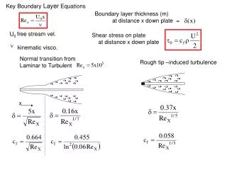
25. NOMINAL BOUNDARY LAYER THICKNESS Until now we have not given a precise definition for boundary layer thickness. Use  to denote nominal boundary thickness, which is defined to be the value of y at which u = 0.99 U, i.e. The choice 0.99 is arbitrary; we could have chosen 0.98 or 0.995 or whatever we find reasonable.

26. Streamwise Variation of Boundary Layer Thickness Consider a plate of length L. Based on the Boundary Layer Approximations, maximum value of  is estimated as Similarly the local value of  is estimated as