Download

1 / 40
400 likes | 485 Views
Explore the theory and methods behind analyzing flat plate boundary layer flows for mechanical engineering applications, focusing on understanding pure wall effects and similarity solutions. Discover how to convert boundary layer equations into eligible forms and solve for similarity variables to determine velocity profiles.

E N D
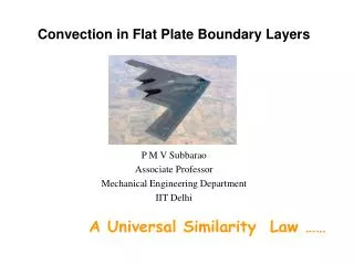
Analysis of Flat Plate Boundary Layer flows P M V Subbarao Professor Mechanical Engineering Department I I T Delhi Understand Pure Wall Effects under in Perceivable Fluid Flows …..…
FLAT PLATE BOUNDARY LAYER EQUATIONS SIMILARITY At all x > 0
Similarity Of Velcoity Profiles (x) is the local boundary layer thickness. Suppose the solution has the property that when u/U is plotted against y/, a universal function is obtained, with no further dependence on x. Such a solution is called a similarity solution. Similarity is satisfied if a plot of u/U versus y/ defines exactly the same function regardless of the value of x. Similarity satisfied Similarity not satisfied
Discovery of SIMILARITY Variable For a solution obeying similarity in the velocity profile we must have where f1 is a universal function, independent of x (position along the plate). Since we have reason to believe that We can rewrite any such similarity form as Note that is a dimensionless variable.
Approximate Analytical Method -1 • Polhausen Approximate Solution
Are these Equations Eligible for Similarity Solution Maybe, maybe not, you never know , Try to convert these equations into an eligible form. Introduce Stream function,(x,y). Note that the stream function satisfies continuity identically.
Discovery of Similarity Variable by The Method Of Guessing We want our stream function to give us a velocity u = /y satisfying the similarity variable So we could start-off by guessing Along with a similarity function for velocity profile where F is a similarity function. Will it work ???? Lets see….. so that
Is it a right Guess ? If we assume not OK OK then we obtain This form does not satisfy the condition that u/U is a function of alone. Similarity demands the first derivative F’() is to be a function of alone, but not F. But note the extra function in x via the term (Ux)-1/2! So our first guess failed because of the term (Ux)-1/2. Use this guess to generate a better guess.
Second Guess learnt from the first Guess This time we assume Now remembering that x and y are independent of each other and recalling the evaluation of /y, Thus the first guess helped in guessing the correct function this new form of that satisfies similarity in velocity! But this does not mean that we are done. We have to solve for the function F().
The Basic of Similarity Variable Our goal is to reduce the partial differential equation using and . To do this we will need the following basic derivatives:
Conversion of Third Order PD into OD The next steps involve tedious differential calculus, to evaluate the terms in the BL Stream Function equation. The third order Partial derivative is:
Conversion of Second Order PDs into ODs we now work out the two second order derivatives:
BOUNDARY CONDITIONS The boundary conditions are But we already showed that
The Blasius Equation • The Blasius equation with the boundary conditions exhibits a boundary value problem. • However, the location of one boundary is unknown, though boundary condition is known. • However, using an iterative method, it can be converted into an initial value problem. • Assuming a certain initial value for F=0, Blasius equation can be solved using Runge-Kutta or Predictor- Corrector methods
FF'F'' 0 0 0 0.33206 0.1 0.00166 0.03321 0.33205 0.2 0.00664 0.06641 0.33199 0.3 0.01494 0.0996 0.33181 0.4 0.02656 0.13277 0.33147 0.5 0.04149 0.16589 0.33091 0.6 0.05974 0.19894 0.33008 0.7 0.08128 0.23189 0.32892 0.8 0.10611 0.26471 0.32739 0.9 0.13421 0.29736 0.32544 1 0.16557 0.32978 0.32301 1.1 0.20016 0.36194 0.32007 1.2 0.23795 0.39378 0.31659 1.3 0.27891 0.42524 0.31253 1.4 0.32298 0.45627 0.30787 1.5 0.37014 0.48679 0.30258 1.6 0.42032 0.51676 0.29667 1.7 0.47347 0.54611 0.29011 1.8 0.52952 0.57476 0.28293 1.9 0.5884 0.60267 0.27514 2 0.65003 0.62977 0.26675 Runge’s Numerical Reults
FF'F'' 2.2 0.7812 0.68132 0.24835 2.3 0.85056 0.70566 0.23843 2.4 0.9223 0.72899 0.22809 2.5 0.99632 0.75127 0.21741 2.6 1.07251 0.77246 0.20646 2.7 1.15077 0.79255 0.19529 2.8 1.23099 0.81152 0.18401 2.9 1.31304 0.82935 0.17267 3 1.39682 0.84605 0.16136 3.1 1.48221 0.86162 0.15016 3.2 1.56911 0.87609 0.13913 3.3 1.65739 0.88946 0.12835 3.4 1.74696 0.90177 0.11788 3.5 1.83771 0.91305 0.10777 3.6 1.92954 0.92334 0.09809 3.7 2.02235 0.93268 0.08886 3.8 2.11604 0.94112 0.08013 3.9 2.21054 0.94872 0.07191
FF'F'' 4 2.30576 0.95552 0.06423 4.1 2.40162 0.96159 0.0571 4.2 2.49806 0.96696 0.05052 4.3 2.595 0.97171 0.04448 4.4 2.69238 0.97588 0.03897 4.5 2.79015 0.97952 0.03398 4.6 2.88827 0.98269 0.02948 4.7 2.98668 0.98543 0.02546 4.8 3.08534 0.98779 0.02187 4.9 3.18422 0.98982 0.0187 5 3.2833 0.99155 0.01591 5.1 3.38253 0.99301 0.01347 5.2 3.48189 0.99425 0.01134 5.3 3.58137 0.99529 0.00951 5.4 3.68094 0.99616 0.00793 5.5 3.7806 0.99688 0.00658
FF'F'' 5.6 3.88032 0.99748 0.00543 5.7 3.98009 0.99798 0.00446 5.8 4.07991 0.99838 0.00365 5.9 4.17976 0.99871 0.00297 6 4.27965 0.99898 0.0024 6.1 4.37956 0.99919 0.00193 6.2 4.47949 0.99937 0.00155 6.3 4.57943 0.99951 0.00124 6.4 4.67939 0.99962 0.00098 6.5 4.77935 0.9997 0.00077 6.6 4.87933 0.99977 0.00061 6.7 4.97931 0.99983 0.00048 6.8 5.07929 0.99987 0.00037 6.9 5.17928 0.9999 0.00029 7 5.27927 0.99993 0.00022
FF'F'' 7.1 5.37927 0.99995 0.00017 7.2 5.47926 0.99996 0.00013 7.3 5.57926 0.99997 9.8E-05 7.4 5.67926 0.99998 7.4E-05 7.5 5.77925 0.99999 5.5E-05 7.6 5.87925 0.99999 4.1E-05 7.7 5.97925 1 3.1E-05 7.8 6.07925 1 2.3E-05 7.9 6.17925 1 1.7E-05 8 6.27925 1 1.2E-05 8.1 6.37925 1 8.9E-06 8.2 6.47925 1 6.5E-06 8.3 6.57925 1 4.7E-06 8.4 6.67925 1 3.4E-06 8.5 6.77925 1 2.4E-06 8.6 6.87925 1 1.7E-06 8.7 6.97925 1 1.2E-06 8.8 7.07925 1 8.5E-07
NOMINAL BOUNDARY LAYER THICKNESS Recall that the nominal boundary thickness is defined such that u = 0.99 U when y = . By interpolating on the table, it is seen that u/U = F’ = 0.99 when = 4.91. Since u = 0.99 U when = 4.91 and = y[U/(x)]1/2, it follows that the relation for nominal boundary layer thickness is FF'F'' 4.6 2.88827 0.98269 0.02948 4.7 2.98668 0.98543 0.02546 4.8 3.08534 0.98779 0.02187 4.9 3.18422 0.98982 0.0187 5 3.2833 0.99155 0.01591 5.1 3.38253 0.99301 0.01347
DRAG FORCE ON THE FLAT PLATE Let the flat plate have length L and width b out of the page: b L The shear stress o (drag force per unit area) acting on one side of the plate is given as Since the flow is assumed to be uniform out of the page, the total drag force FD acting on the plate is given as The term u/y = 2/y2is given from as
The shear stress o(x) on the flat plate is then given as FF'F'' 0 0 0 0.33206 0.1 0.00166 0.03321 0.33205 0.2 0.00664 0.06641 0.33199 0.3 0.01494 0.0996 0.33181 0.4 0.02656 0.13277 0.33147 0.5 0.04149 0.16589 0.33091 But from the table F (0) = 0.332, so that boundary shear stress is given as Thus the boundary shear stress varies as x-1/2. A sample case is illustrated on the next slide for the case U = 10 m/s, = 1x10⁻⁶ m2/s, L = 10 m and = 1000 kg/m3 (water).
Variation of Local Shear Stress along the Length Sample distribution of shear stress o(x) on a flat plate: U = 0.04 m/s L = 0.1 m = 1.5x10⁻⁵ m2/s = 1.2 kg/m3 (air) Note that o = at x = 0. Does this mean that the drag force FD is also infinite?
DRAG FORCE ON THE FLAT PLATE The drag force converges to a finite value!
Similarity of An evolving FBL • The application of integral balances to the control volume shown in above figure delivers more similarity features. • the boundary layer displacement thickness • the boundary layer momentum deficiency thickness and • the energy deficiency thickness .
Impermeable Streamlines of A BL • The lower side should be the wall itself; hence the drag force will be exposed. • The upper side should be a streamline outside the shear layer, so that the viscous drag is zero along this line.
Integral View of A FPBL • Integral Method
Using continuity equation : The partial integration of the second term of the left side of above equation gives:
The Displacement Thickness Assuming incompressible flow, this relation simplifies to • Conservation of mass is applied to this Engineering CV @SSSF:
* is the engineering formal definition of the boundary-layer displacement Thickness and holds true for any incompressible flow.
Physical Interpretation of Momentum and displacement thicknesses The ratio of displacement thickness to momentum thickness is called the shape factor, is often used in boundary-layer analyses: