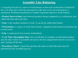
Assembly Line Balance

Assembly Line Balance Balance

Assembly analysis Assembly Chart It shows the sequence of operations in putting the product together. Using the exploded drawing and the parts list, the layout designer will diagram the assembly process. The sequence of assembly may have several alternatives. Time standards are required to decide which sequence is best. This process is known as assembly line balancing. Balance

The Assembly Chart The assembly chart of a toolbox Balance

Time Standards Are Required for Every Task Balance

Plant Rate and Conveyor Speed Conveyor speed is dependent on the number and units needed per minute, the size of the unit, the space between units. Conveyor belt speed is recorded in feet per minute. Example: Charcoal grill are in cartons 30X30X24 inches high. A total of 2,400 grills are required every day. Balance

Plant Rate and Conveyor Speed Balance

Assembly line balancing The purpose of the assembly line balancing technique is: 1. To equalize the work load among the assemblers 2. To identify the bottleneck operation 3. To establish the speed of the assembly line 4. To determine the number of workstations 5.To determine the labor cost of assembly and packout 6. To establish the percentage workload of each operator 7. To assist in plant layout 8. To reduce production cost The assembly line balancing technique builds on: The assembly chart; Time standards; Takt time (minutes/piece) (Plant rate, R value, Pieces/minutes). Balance

Initial assembly line balancing of toolbox Takt time (for 2,000 units per shift, considering 10% downtime and 80% efficiency) = .173 minutes per unit. Balance

Assembly line balancing • Cost of balancing • Subassemblies that cost too high can be taken off the line. • SA3 could be taken off the assembly line and handled completely separate from the main line and we can save money. SA3 .250 = 240 pieces per hour and .00417 hour each. If balanced, the standard would be 180 pieces per hour and .00557 hour each. • .0057 balanced cost • - .00417 by itself cost • .00140 savings hour per unit • X 500,000 units per year • 700 hours per year • @ $15.00per hour • = $10,500.00 per year savings Balance

Assembly line balancing Subassemblies that can be taken off the line must be: 1. Poorly loaded. The less percent that is loaded. For example, a 60 percent load on the assembly line balance would indicate 40 percent lost time. If we take this job off the assembly line (not tied to the other operators), we could save 40 percent of the cost. 2. Small parts that are easily stacked and stored. 3. Easily moved. The cost of transportation and the inventory cost will go up, but because of better labor utilization, total cost must go down. Balance

Assembly line balancing 2. Improvement of assembly line Improve the busiest (100 percent) workstation first. (a) The busiest workstation is P.O. It has .167 minute of work to do per packer. The next closest station is A1 with .155 minute of work. As soon as we identify the busiest workstation, we identify it as the 100 percent station, and communicate that this time standard is the only time standard used on this line from now on. Every other workstation is limited to 360 pieces per hour. Even though other workstations could work faster, the 100 percent station limits the output of the whole assembly line. (b) The total hours required to assemble one finished toolbox is .06960 hour. The average hourly wage rate times .06960 hour per unit gives us the assembly and packout labor cost. Again, the lower this cost is the better the line balance is. Balance

Assembly line balancing Balance

Assembly line balancing 2. Improvement of assembly line Improve the busiest (100 percent) workstation first. Look at the 100 percent station (P.O.). If we add a fourth packer, we will eliminate the 100 percent station at P.O. Now the new 100 percent (bottleneck station) is A1 (93 percent). By adding this person, we will save 7 percent of 25 people or 1.75 people and increase the percent load of everyone on the assembly line (except P.O.). We might now combine A1 and A2, and further reduce the 100 percent. The best answer to an assembly line balance problem is the lowest total number of hours per unit. If we add an additional person, that person’s time is in the total hours. Balance

Step-by-step procedure for completing the assembly line balancing form Balance

Step-by-step procedure for completing the assembly line balancing form 9. R value The R value goes behind each operation. The plant rate is the goal of each workstation, and by putting the R value on each line (operation), one keeps that goal clearly in focus. 10. Cycle time The time standard. 11. Number of stations 12. Average cycle time Balance

Step-by-step procedure for completing the assembly line balancing form 13.Percentage load: The percentage load tells how busy each workstation is compared to the busiest workstation. The highest number in the average cycle time column 12 is the busiest workstation and, therefore, is called the 100 percent station. Now every other station is compared to this 100 percent station by dividing the 100 percent average station time into every other average station time. The percent load is an indication of where more work is needed or where cost reduction efforts will be most fruitful. if the 100 percent station can be reduced by 1 percent, then we will save 1 percent for every workstation on the line. Balance

Step-by-step procedure for completing the assembly line balancing form 13.Percentage load: Example: percent load of the toolbox assembly line balance In Figure 4-11, the average cycle times reveals that .167 is the largest number and is designated the 100 percent workstation. The percentage load of every other workstation is determined by dividing .167 into every other average cycle time: Operation SSSA1 = .153 / .167 = 92 percent SSA1 = .146 / .167 = 87 percent SSA2 = .130 / .167 = 78 percent and so on. Balance

Step-by-step procedure for completing the assembly line balancing form 14.Hours per unit: Example: Hours per unit of the toolbox assembly line balance The .167 time standard is for one person, if considering the people number, the hour per unit will be: Two people = .00557 hour per unit Three people = .00835 hour per unit Four people = .01113 hour per unit Balance

Step-by-step procedure for completing the assembly line balancing form 15. Piece per hour: Inversion of hours per unit. 16. Total hours per unit Sum of the elements in column 14. For this example is .0696 hour. 17. Average hourly wage rate, say $15 per hour 18. Labor cost per unit Total hours X average hourly wage 19. Total cycle time It tells us what a perfect line balance would be. Our example 3.494 minutes divided by 60 minutes per hour equals .05823 hour per unit. Balance

Efficiency of the assembly line or For our example: Balance

Analysis of single model assembly lines Production Rate is given by where Rp = average hourly production rate, units/hr; Da = annual demand, units/year; Sw= number of shifts/week; Hsh = hrs/shift. This equation assume 50 weeks per year. Balance

Analysis of single model assembly lines The cycle time can be determined as where Tc = cycle time of the line, min./cycle; Rp = production rate, units/hr; E = line efficiency; Balance

Analysis of single model assembly lines The cycle rate can be determined as where Rc = cycle rate, cycles/hr; Tc is in min./cycle; Line efficiency E therefore defined as: Balance

Analysis of single model assembly lines The number of workers on the line can be determined as where w = number of workers on the line; WL = workload to be accomplished in a given time period. AT = available time in the period. TWc = work content time, min/piece. Balance

Analysis of single model assembly lines Using the previous equation, we also have The available time in the period, AT. AT = 60E Substitute these terms for WL and AT into w equation, we can state: If we assume one worker per station, then this ratio also gives the theoretical minimum number of workstations on the line. Balance

Analysis of single model assembly lines Example A small electrical appliance is to be produced on a single model assembly line. The work content of assembling the product has been reduced to the work elements listed in table below along with other information. The line is to be balanced for an annual demand of 100,000 units per year. The line will be operated 50 weeks/yr, 5 shifts/wk, and 7.5 hrs/shift. Manning level will be one worker per station. Previous experience suggests that the uptime efficiency for the line will be 96%, and repositioning time lost per cycle will be 0.08 min. Determine (a) total work content time Twc, (b) required hourly production rate Rp to achieve the annual demand, (c) Cycle time, and (e) service time Ts to which the line must be balanced. Balance

Analysis of single model assembly lines Example Balance

Analysis of single model assembly lines Solution: • The total work content time is: • Twc= 4.0 min. (b) The production rate is: (c) The cycle time Tc with an uptime efficiency of 96% is: Balance

Analysis of single model assembly lines Solution: (d) The theoretical minimum number of workers is given by: (e) The average service time against which the line must be balanced is: Balance

Analysis of single model assembly lines The objective in line balancing is to distribute the total workload on the assembly line as evenly as possible among the workers subject to: and (2) all precedence requirements are obeyed. Balance

Analysis of single model assembly lines The algorithms are: Largest Candidate Rule Kilbridge and Wester method Ranked positional weights Balance

Largest Candidate Rule Step 1: Rank the Teks in the descending order. Step 2: Assign the elements to the worker at first station by starting at the top of the list and selecting the first element that satisfies precedence requirements and does not cause the total sum of Tek at that station to exceed the allowable Ts; when an element is selected for assignment to the station, start back at the top of the list for subsequent assignments. Step 3: when no more element can be assigned without exceeding Ts, then proceed to the next station. Step 4: repeat steps 2 and 3 for as many additional stations as necessary until all elements have been assigned. Balance

Largest Candidate Rule Work elements sorted in descending order Balance

Largest Candidate Rule Solution: The largest candidate algorithm is carried out as presented in table below. 5 workers and stations are required in the solution. Balance efficiency is computed as: Balance

Largest Candidate Rule Work elements assigned to stations by LCR Balance

Analysis of single model assembly lines Example Balance

Analysis of single model assembly lines Kilbridge and Wester method Balance

Analysis of single model assembly lines Ranked positional weights Balance

Analysis of single model assembly lines Ranked positional weights Largest Candidate Rule Kilbridge and Wester method Balance

Analysis of single model assembly lines • Automation, Production Systems, and Computer-Integrated Manufacturing, By Mikell P. Groover, 3rd edition, c2008. • Manufacturing Facilities Design and Material Handling, By F. E. Meyers and M. P. Stephens, 4th Edition, Prentice-Hall, Inc., 2010 Balance

Assembly Line Balance