Download
1 / 33
350 likes | 546 Views
Larmor-resonant Sodium Excitation for Laser Guide Stars. Ron Holzlöhner S. Rochester 1 D. Budker 2,1 D. Bonaccini Calia ESO LGS Group 1 Rochester Scientific LLC, 2 Dept. of Physics, UC Berkeley. AO4ELT3 Florence, 28 May 2013. Are E-ELT LGS lasers powerful enough?.

E N D
Larmor-resonant Sodium Excitation for Laser Guide Stars Ron Holzlöhner S. Rochester 1 D. Budker 2,1 D. BonacciniCalia ESO LGS Group 1 Rochester Scientific LLC, 2 Dept. of Physics, UC Berkeley AO4ELT3 Florence, 28 May 2013
Are E-ELT LGS lasers powerful enough? • E-ELT laser baseline: 20W cw with 12% repumping 5 Mph/s/m2 at Nasmyth (at zenith in median sodium; 12 Mph/s/m2 on ground) • There may be situations when flux is not sufficient for some instruments (low sodium, large zenith angle, non-photometric night, full moon, etc.) • No unique definition of LGS availability; details quite complicated • E-ELT Project has expressed interest in exploring paths to raise the return flux • Two avenues: • Raise cw power Laser development (e.g., Raman fiber amplifiers) • Raise coupling efficiency sce Explore new laser formats • Will focus on option 2
Sky Maps Paranal • Becoming more independent of field angle would be particularly beneficial in Paranal: • Flux varies strongly with angle to B-field • B-field inclination is only 21° most of the time this angle is large Sim. cw return flux on ground [106 ph/s/m2] B ζ = 60° 3.6!
What factors limit the return flux? B m v θ Laser + 50 kHz spont. emission time excited (P3/2) ground (S1/2) Three major impediments of sodium excitation: 1) Larmor precession (m: angular momentum z-component) 2) Recoil (radiation pressure) 3) Transition saturation (at 62 W/m2 in fully pumped sodium)
z z z y y y x x x Unpolarized Sphere centered at origin, equal probability in all directions. Oriented “Pumpkin” pointing in z-direction preferred direction. Aligned “Peanut” with axis along z preferred axis. Visualization of Atomic Polarization Draw 3D surface where distance from origin equals the probability to be found in a stretched state (m = F) along this direction. Credit: D. Kimball, D. Budker et al., Physics 208a course at UC Berkeley
Precession in Magnetic Field torque causes polarized atoms to precess: B Credit: D. Kimball, D. Budker et al., Physics 208a course at UC Berkeley Credit: E. Kibblewhite
Efficiency per Atom with Repumping Peak efficiency • Model narrow-line cw laser, circular polarization • ψ: Return flux per atom, normalized by irradiance [unit ph/s/sr/atom/(W/m2)] • θ: angle of laser to B-field (design laser for θ = π/2) • Symbols: Monte Carlo simulation, lines: Bloch • Blue curve peaks near 50 W/m2, close to Na saturation at 60 W/m2: Race to beat Larmor Irradiance (W/m2) 20W cw laser in mesosphere Transition saturation 62 W/m2 Is there a way to harness the efficiency at peak of green curve?
Larmor Resonant Pulsing *) PNAS 10.1073/pnas.1013641108 (2011) (arXiv:0912.4310) • Pulse the laser resonantly with Larmor rotation: like stroboscope, Larmor period: 3 – 6.2 μs (Field in Paranal: 0.2251G at 92km) • Used for optical magnetometry: Yields bright resonance in D2a of about 20% at 0.3…1.0 W/m2, narrow resonance of ca. 1.5% FWHM *) • Recent proposal by Hillman et al. to pulse at 9% duty cycle, 20W average power, 47/0.09 = 522 W/m2 and a linewidth of 150 MHz 47/15 ≈ 3 W/m2/vel.class near optimum avg. power • Paranal simulation: sce = 374 ph/s/W/(atoms/m2), vs. ca. sce ≈ 250 for cw (all at 90° and Paranal conditions) hence about 1.5 times more (!) • sce becomes almost independent of field angle • Increased irradiance also broadens the resonance
Some Simulation Details B = 0.23 G, θ= 90°, q = 9%, 150 MHz linewidth Return is fairly linear vs. irradiance Steady state reached after ca. 50 periods = 300μs (S-damping time)
Simulated Performance Ground States 582 W/m2 Excited States F = m = 2 F = m = 1 Can achieve 14 Mph/s/m2 at 10W, 28 Mph/s/m2 at 20W (D2a+D2b) Peak efficiency reached above 10W Very strong atomic polarization towards (F=m=2) of 60–70%
Larmor Detuning On resonance 1% detuned 2% detuned Ip = 221 W/m2 Ip = 27 W/m2 A small rep rate detuning shows up first at low peak irradiance Reduces pumping efficiency, induces polarization oscillations Variation in Paranal: –0.22%/year, –0.39%/10km altitude
Best Laser Format? • Lasers with pulses of ~0.5 μs and peak power 200W hard to build (150/2=75 MHz linewidth not large enough to sufficiently mitigate SBS) • Multiplex cw laser to avoid wasting beam power? • Spatiotemporally: use one laser to sequentially produce multiple stars • In frequency: Chirp laser continuously, e.g. from –55... +55 MHz (11 vel.c.) • In frequency: Periodically address several discrete velocity classes • Or modulate the polarization state? (probably less beneficial) • Can in principle profit from “snowplowing” by up-chirping, although chirp rate of ~110 MHz/6.2μs = 17.7 MHz/μs is very high • Numerical optimization of modulation scheme; runs are time-consuming (order 48–72 CPU h per irradiance step) • Issue: Avoid F=1 downpumping, in particular at 60 MHz offset
Downpumping 3S1/2 3P3/2 transition F = I + J : Total angular momentum I= 3/2 : Nuclear spin J = L + S : Total electronic angular momentum (sum of orbital and spin parts) 40 MHz grid D2b Excitation from D2a narrow-band laser Graphic by Unger D2a Prefer (F = 2, m = ±2) (F = 3, m = ±3) cycling transition
Frequency Scanning Schemes 9 × 40 MHz 4 × 110 MHz Scan across >= 9 discrete velocity classes Blue-shift to achieve “snowplowing” via atomic recoil Avoid downpumping leave 40 MHz or >> 60 MHz gaps, but… …without exceeding the sodium Doppler curve (1.05 GHz FWHM)
Hyperfine State Populations Excitation F = 1 ground states • Plot hyperfine state evolution for a selection of velocity classes • Visualize Larmor precession, downpumping, excitation F = 2 ground states Time excited states Larmor period first pulse
Conclusions CW laser format is good, but leaves room for improvement Larmor precession reduces the return flux efficiency by factor 2; forces high irradiance to combat population mixing Can mitigate population mixing by stroboscopic illumination resonant with Larmor frequency (~160 kHz in Chile, ~330 kHz in continental North America and Europe) Realize with pulsed laser of ~20W average power and < 10% duty cycle, 150 MHz linewidth: Raise efficiency by factor 1.5 ! …which is hard to build (> 200 W peak power, M2 < 1.1) Alternative: Frequency modulation (chirping/frequency multiplexing schemes) Caveats: Observe 60 MHz downpumping trap and target ~3–5 W/m2/v.c. on time average, frequency sensitive, modulator not easy to build Format optimization is work in progress
F I N EGrazie! Slide 18
Frequency Shifters Would like to frequency modulate over 100 MHz (or even 300 MHz) at >80% efficiency Either sawtooth or step function with 160 kHz rep rate (Paranal) Need to maintain excellent beam quality and beam pointing Option1: Free-space AOM. Pro: Proven technique, reasonable efficiency. Con: 100+ MHz is very broadband, variation of beam pointing or position when changing frequency? Option 2: Free-space EOM using carrier-suppressed SSB. Requires an interferometric setup, may be difficult to realize at high power+efficiency Option 3: Modulate seed laser. Pro: Possibly reduce SBS (fiber transmission time is in μs range). Con: Cavity locking difficult (piezo bandwidth would need to be in MHz range), combine with PDH sidebands?
Some Commercial Frequency Shifters 1 Brimrose Corp. http://www.brimrose.com/pdfandwordfiles/aofshift.pdf
Some Commercial Frequency Shifters 2 Brimrose Corp. http://www.brimrose.com/pdfandwordfiles/aofshift.pdf
Some Commercial Frequency Shifters 3 A.A http://opto.braggcell.com/index.php?MAIN_ID=102
To Frequency Shift, or not? Egg-laying wool milk swine: Broadband, highly efficient, high power, no aberrations, constant pointing. And cheap! • Seems that AOM/EOM specs are very challenging (no “eierlegendeWollmilchsau” in AOMs, quote by Mr. Jovanovic, Pegasus Optik GmbH) • Really no way to modulate in the IR and double? • Frequency shift is doubled, hence +/– 25 MHz may be enough • Could be done after seed laser with fiber-coupled AOM and thus also shift the PDH sidebands • Would need fast adjustment of optical path length in cavity (RF active crystal? LBO not suitable, but has been done e.g. with MgO:LiNbO3) • …or else consider a pulsed laser?
Bloch Equation Simulation Schrödinger equation of density matrix, first quantization dρ/dt = Aρ + b = 0 Models ensemble of sodium atoms, 100–300 velocity groups Takes into account all 24 Na states, Doppler broadening, spontaneous and stimulated emission, saturation, collisional relaxation, Larmor precession, recoil, finite linewidth lasers Collisions change velocity and spin (“v-damping,S-damping”) More rigorous and faster than Monte Carlo rate equations Based on AtomicDensityMatrix package, http://budker.berkeley.edu/ADM/ Written in Mathematica v.6+, publicly available [“Optimization of cw sodium laser guide star efficiency”, Astronomy & Astrophysics 520, A20]
EOMs for Repumping • Vendors: New Focus, Qubig • Used free-space EOM in “Wendelstein” transportable LGS system • Issues with peak power (photodarkening, coatings, cooling) Taken from www.qubig.de Affordable way to retrofit pulsed lasers
What is crucial for good return flux? Could improve on the crucial parameters (☼) Most Important: Laser power, sodium abundance (seasonal) Circular polarization state ☼ D2b repumping (power fraction q≈12%, 1.710 GHz spacing) ☼ (Peak) power per velocity class ☼ Overlap with sodium Doppler curve (but: implicit repumping) ☼ For return flux on ground: zenith angle, atmospheric transmission2 Somewhat Important: Angle to B-field (θ), strength of B-field |B| (hence geographic location) Atomic collision rates (factor 10 variation across mesosphere) Less Important: Seeing, launched wavefront error, launch aperture (beware: spot size) Sodium profile, spectral shape (for given number of velocity classes)
Optical pumping Light linearly polarized along z can create alignment along z-axis. z F’ = 0 F = 1 MF = -1 MF = 0 MF = 1 Credit: D. Kimball, D. Budker et al., Physics 208a course at UC Berkeley http://budker.berkeley.edu/Physics208/D_Kimball/
Optical pumping Light linearly polarized along z can create alignment along z-axis. z F’ = 0 F = 1 MF = -1 MF = 0 MF = 1 Medium is now transparent to light with linear polarization along z ! Credit: D. Kimball, D. Budker et al., Physics 208a course at UC Berkeley
. Optical pumping Light linearly polarized along z can create alignment along z-axis. z F’ = 0 F = 1 MF = -1 MF = 0 MF = 1 Medium strongly absorbs light polarized in orthogonal direction! Credit: D. Kimball, D. Budker et al., Physics 208a course at UC Berkeley
Optical pumping Optical pumping process polarizes atoms. Optical pumping is most efficient when laser frequency (l) is tuned to atomic resonance frequency (0).
= B = B dF = dt dF = B = gFB F B dt Precession in Magnetic Field Interaction of the magnetic dipole moment with a magnetic field causes the angular momentum to precess – just like a gyroscope! B , F L = gF B B