Download
1 / 47
550 likes | 1.08k Views
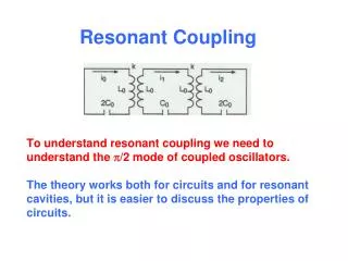
To understand resonant coupling we need to understand the p /2 mode of coupled oscillators. The theory works both for circuits and for resonant cavities, but it is easier to discuss the properties of circuits. . Resonant Coupling. Three Coupled Oscillators.

E N D
To understand resonant coupling we need to understand the p/2 mode of coupled oscillators.The theory works both for circuits and for resonant cavities, but it is easier to discuss the properties of circuits. Resonant Coupling
Three Coupled Oscillators • Begin with a three-oscillator system of electrical circuits to get an understanding of the physics of coupled oscillators. • First look at the steady-state harmonic solutions of three identical electrical oscillators with no power losses.
Three Coupled Oscillators(cont) • First, we write Kirchoff’s equations for each oscillator with no power losses and find the three steady-state modes, their resonant frequencies, and corresponding eigenvectors (containing individual oscillator amplitudes and phases). • Later, we introduce local oscillator frequency errors and use perturbation theory to see how the mode frequencies and eigenvectors are modified. • Finally, we introduce power losses(adding an RF generator to supply the losses) and see how this affects the mode frequencies and eigenvectors.
Complex exponential notation is helpful • Harmonic time dependence is represented by exp(jwt) time dependence where wt is the phase at time t. • Recall Re[exp(jwt)]=Re[cos(wt)+jsin(wt)=cos(wt) • If B=A exp(jf), it means the phase of B is larger than the phase of A by f. • Another relationship: exp(jp/2)=cos(p/2)+jsin(p/2)=j. Thus j represents a phase increase of p/2. • Thus j= exp(jp/2] and j exp(jwt)=exp(j[wt+p/2].
Solve for three steady-state modes • Procedure is to solve an “eigenvalue problem”. The three Kirchoff’s • equations can be expressed in the following form. • Eigenvector components give the currents in each cell.We find • Want solutions for Xq and Wq. There will be 3 solutions (3 modes).
Eigenvalue problem results for the three modes • Three steady-state modes k is proportional to mode freq spread
These are steady-state results for ideal conditions with no cell-frequency errors and no power losses. • What happens when we introduce small • resonant-frequency errors in individual cells?
dw1 +dw0 w0 -dw0 cell0 cell 1 cell2 Perturbation Theory • Suppose the cells are slightly different, i.e. suppose we introduce errors. • In the unperturbed case all the cells have the same frequency w0. • In the perturbed case the three frequencies will be slightly different and experimentally we don’t have any way to define the unperturbed frequency. • Let’s make it easy for ourself. No generality is lost in the perturbed case by defining the unperturbed frequency w0 to equal the average of the two end cell frequencies. • Then the two end cell frequency errors are –dw0 and +dw0. The middle cell frequency error is called dw1.
Perturbation theory corrections for mode q-first order theory • Note amplitudes aqr are larger for modes r close in frequency to mode q.
Perturbation Theory Results • Corrections • Are linear inthe errors. • Correctionsare quadratic for • the errors in end • cells in p/2 mode • so they are very • small.
Perturbation Theory Results (2) • Correctionsare linear in theerrors. • There are first-order corrections to mode frequency and eigenvectors in the0 and p modes. • We have included second order terms for p/2 mode when the first order termswere zero. • Notice the p/2 mode is different from the other two modes. The frequency and end-cell amplitudes have only second-order corrections. Thus, the p/2-mode end-cell amplitudes are very insensitive to cell frequency errors.
Effects of cell errors in perturbation theory • Corrections for 0 and p mode frequencies and oscillator amplitudes are first order in the local or cell frequency errors. • Notice the p/2 mode is different. The mode frequencies and end cell amplitudes have only second-order corrections from the cell frequency errors. Local frequency errors are much less important for p/2 mode. • Can the insensitivity of the p/2 mode to cell frequency errors can be used to advantage for accelerating structures?
Next, turn off the cell errors and turn on power losses. What happens to the mode frequency and the eigenvectors?
Effects of Power Dissipation in Steady State • Turn off cell frequency errors, turn on power losses, and turn on thegenerator to supply the power losses. • Assume the generator is in cell 0.Q is the quality factor. The results are: • Power flow droop and power flow phase shift are so named because 1/Q is proportional to power P.
Effects of power dissipation on cell amplitudes and phases • No amplitude change for the 0 and p modes but one has phase shifts in cells downstream of the drive point that are first order in 1/kQ, called power-flow phase shifts. • The p/2 mode is different with power loss. Not just phase shifts. The middle cell is now excited. • Also, the excited end cell in the p/2 mode has a second order amplitude correction, called power flow droop. Because it is second order this effect is very small.
Summary of the Three Coupled Oscillator Problem • The analysis reveals sensitivity to cell frequency errors for the 0 and p mode. • Power flow from the generator to the other cells in the array causes phase shifts in 0 and p mode. • The excited end cells in the p/2 mode are insensitive to both cell frequency errors and power loss. • Question: How will these results carry over to the general problem of N coupled oscillators?
C0 2C0 C0 2C0 General results for N+1 Coupled Oscillators • Dispersion curve is mode frequency Wq versus phase advance per cell pq/N. • Eigenvectors (fields):
Bandwidth=Dw=kw0 p/2 p 0 Example: Dispersion Curve (mode frequency versus phase advance per cell) in this case for 7 coupled oscillators, i.e. N=6. The p/2 mode is in the middle.
How to use the p/2 mode for an accelerating structure • The p/2 mode has unique properties that are related fundamentally to its central location in the mode spectrum. • Fields in the excited cells are insensitive to cell frequency errors. • We could use the p/2 mode for an accelerating structure by using the excited cells for acceleration, and designing these cells with a spacing bl/2 as you would for p mode. • Then the synchronous particle will arrive at the right time for continued acceleration.
Need to improve the p/2 mode efficiency for an accelerating structure • The problem for p/2 mode is poor efficiencycompared with the 0 or p mode(or the other non-p/2 modes)if the beam passes through the nominally unexcited cells, since these cells do not contribute any acceleration.
Power inefficiency for p/2 mode of a periodic structure relative to p mode For example consider a long periodic array of cells with equal cell lengths for all cells. In a given structure length the p/2 mode structure must have twice the field in the excited cells to deliver the same energy to the beam as the p mode. Then, as is illustrated below, twice as much power is dissipated in the p/2 mode than for the 0 or p mode. Two cells in p mode Two cells in p/2 mode Field : E E 2E 0 Relative power loss : P=E2+E2=2E2 P=(2E)2=4E2
Solutions to improve the p/2 mode efficiency for an RF accelerating structure • We could improve the efficiency of the p/2 mode by using different cell types for the accelerating and coupling cells, i.e. reduce size of coupling cells. • An even more attractive solution is tomove the unexcited cells completely off to the sideresulting in a “side-coupled” structure.
Evolution to p/2 mode for the side-coupled structure • p/2 mode of a periodic structure.Half the space is inactive due tothe unexcited coupling cells.(Periodic structure) • Can decrease the inactive volume of the coupling cells to improve theefficiency. (On-axis coupled structure) • Or we can remove the coupling • cavities to the sides so beam sees • only the accelerating cells in a • “p-mode” configuration, whereas • electrically the structure is in a • p/2 mode. (Side-coupled structure)
p/2-mode biperiodic structures produce stable field distributions for long multicell structures.This is the approach used for long normal-conducting coupled-cavity linacs at high velocities (b>0.5). Side-coupled linac structure Cavities on the side are nominally unexcited coupling cavities.
Side-Coupled Linac Structure Showing Accelerating Cells and Coupling Cells D. Nagel, E. Knapp, and B. Knapp, Rev. Sci. Instrum. 38, 1583-1587 (1967)
wp Upper p/2 modecan be excited wa wc Lower p/2 mode forbidden because of boundary condition w0 p p/2 0 Modes in a Side-Coupled Linac Structure • Example: 9 cells and 9 modes, 5 accelerating cells and 4 coupling cells Note: For biperiodic structure there are two branches. The cavities must be tuned to remove the gap. Then you get all the desired p/2 mode properties. • 0-mode: • p mode
Physical picture ofallowedand forbidden p/2 modes • The above p/2-mode coupling cell (yellow) is unexcited because it is being • driven by two excited cells (blue) with equal and opposite amplitudes. This is allowed. • The above mode for 9 cells is also allowed, since each unexcited coupling cell has equal and opposite drive signals required to make it unexcited. • This mode is forbidden, since the unexcited end cells have a nonzero driving amplitude and therefore can’t be unexcited.
Focusing is provided in a side-coupled linac by introducing a displaced “accelerating cavity” called a bridge coupler to make room for focusing lenses on the axis. Klystron Accelerating cell Bridge coupler Coupling cell Quadrupole • The bridge coupler functions electrically as an excited cell just like an accelerating cavity, but is off axis to make room for focusing quadrupoles. • The bridge coupler may also be used for the drive cell, as shown in the figure.
Resonant Coupling • The general approach of using resonant oscillators as coupling elements to stabilize the field distribution of a multicell standing-wave cavity is called resonant coupling. • This enables construction of long multicell linac structures, providing advantages for simplicity and reduced cost for many linac applications. • Two examples of normal-conducting ion linacs that incorporate resonant coupling: 1) Side-coupled linac 2) Post-coupled DTL
Example 1: Side-Coupled Linac Structure Showing Accelerating Cells and Coupling Cells The side-coupled linac is used at LANSCE linac at Los Alamos and in the SNS linac at Oak Ridge.
Example 2: Alvarez drift-tube linac • Basic Alvarez drift-tube linac (DTL) showing drift tubes and supporting stems. The DTL operates in a 0 mode (or equivalently a 2p mode) in which all the cells are in phase. • However, for long DTLs the fields are very sensitive to local frequency errors.
Post-couplers are used for resonantcoupling in the drift-tube-linac structure (D. Swenson) The resonant-coupling elements for the DTL are internal posts, called post couplers. These are quasi-coaxial resonators tuned by radial positioning to have electrical length l/4. Post couplers are used in the LANSCE DTL at Los Alamos and in the SNS linac at Oak Ridge.
Post-coupler stabilizes the fields in the accelerating cells. • Post couplers mount on cylindrical wall across from the center of each drift tube. The posts are tuned to the RFQ frequency and are nominally unexcited. • Posts extend radially inward leaving a small gap near the body of each drift tube. • Each post may be thought of as being capacitively coupled to each end of the opposing drift tube. • Any field unbalance in the two adjacent cells produces a net excitation of the post, which stabilizes the fields as in the 3-coupled oscillator system
Distinctive feature of post-coupled DTL • Unlike the coupling cavities of the side-coupled linac, in the post-coupled DTL the post fields share the same volume as the DTL accelerating cells.
First example: D. Swenson’s concept for resonant coupling of an RFQ and a DTL • To resonantly couple two resonant cavities it is necessary to introduce a third resonator coupled to both cavities and to tune the assembly to operate in the p/2 mode. In this mode the coupling resonator is nominally unexcited. • In this concept Swenson introduces a quarter-wave post at the point where the RFQ and DTL structures come together. • He couples the post to both the magnetic fields going around the ends of the RFQ vanes, and to the azimuthal magnetic fields of the DTL structure.
Swenson’s RFQ to DTL resonant couplingscheme. The X’s are magnetic field lines. Coupler X X Resonant coupler is coaxiall/4 resonator and is designed to have no net excitation when RFQ and DTL are at nominal field levels. This is necessary for p/2 mode. X X X RFQ DTL beam beam Drift tubes Note that coupler is driven 180 deg out of phase by RFQ and DTL, so if tuned properly the two drives cancel out. X
Objective of resonant coupling of RFQ to DTL • The main idea here is to be able to close-couple the RFQ and DTL, to avoid having to install an RFQ-DTL transition beamline with quads and a buncher, but just go directly from RFQ into the DTL. • A 3D electromagnetic field solver code is a useful tool to optimize the geometry and to test if this works.
Another example: Resonant coupling of pairs of RFQsL.M.Young, “Operations of the LEDA resonantly coupled RFQ”, Proc. of 2001 Part. Accel. Conf., Chicago, 2001, 309-313.
LEDA RFQ 1999 at Los Alamos,100-mA protons CW, 75 keV to 6.7 MeV, 350-MHz, 8-m long, 0.67 MW beam power, three 1 MW klystrons.
LEDA RFQ resonant coupling • A continuous single-segment 8-m-long 350-MHz (l=0.857m) RFQ would be 9.3 wavelengths long, we would be unable to maintain the design intervane voltage distribution. • Instead, four 2-m long RFQ segments (2.3 wavelengths each) are resonantly coupled to form the 8-m long RFQ • Resonant coupling is implemented by separating the four 2-m-long RFQs by coupling plates with an axial hole in them. • Adjusting the gap between the vanes tunes the coupling mode frequency to the RFQ frequency.
beam RFQ1 RFQ2 X B B coupling plate Consider end regions of two RFQs electromagnetically uncoupled by a conducting end plate with a small beam aperture O B • In this picture the two RFQs are uncoupled because of the conducting • plate that divides and electromagnetically separates the RFQs.
-V 0 +V Recipe to resonantly couple these RFQs • Look for a geometry that introduces a coupling resonator to couple the two RFQ resonators. • To provide the desired p/2 mode, the coupling resonator must be -tuned to the same frequency as the RFQs, and must be -unexcited when the two RFQs being coupled are operating at their nominal design values. Equivalent p/2-mode configuration of of three coupled resonators
Modifying the plate to form a resonant coupler • Enlarge the beam aperture of the coupling plate. This creates a gap for capacitance between the coupling plate and the two RFQs. • The resonant coupler not only needs capacitance but also inductance. It shares the same inductive volume of the cutaway end region of each RFQ end cell. • Thus the coupling plate provides capactive gaps to each RFQ vane and the two RFQ undercuts provide inductance.
Enlarged coupling-plate-hole allows plate to couple to both vanetips.There is no net electric field at the aperture of the coupling plate when properly turned and no errors; then coupling resonator is unexcited.Vanetip unbalance excites coupling plate and drives currents to correct the unbalance. beam RFQ1 RFQ2 Resonant coupling plate • The coupling resonator consists of the capacitances between the coupling plate and the vanetips plus the inductances of the vane undercuts. • The gap between vanetips is 3.175 mm.
-V 0 +V This configuration creates a p/2 mode of a three-coupled-resonator system for the LEDA RFQ Equivalent p/2-mode configuration of of the 3 coupled resonators If the currents in the two RFQ end cells are equal there is no net charge on the aperture of the coupling plate. Then the coupling resonator is unexcited. This is the p/2 mode of 3-resonator system. Unbalance of the currents in the two end cells will excite the coupling resonator, and theory predicts that RF power will be driven to compensate for the error.