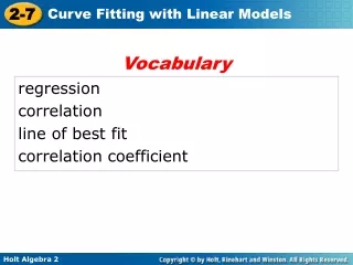

Correlation Coefficient: A Comprehensive Guide
E N D
Presentation Transcript
Correlation coefficient • Housekeeping: • You do not have to read the three articles listed as readings under #14. • You should read the texts, but not the articles. • You do have a short assignment drawn from one of the readings (due 4/14).
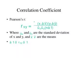
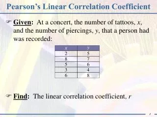
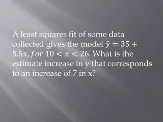
Correlationcoefficient (cont.) • aka Pearson correlation (after its creator, Karl Pearson) and as the product-moment coefficient or correlation • Measures the strength of the association between two interval-level variables as defined by how closely they approximate a straight line. (Recall that lambda, tau, and gamma covered nominal and ordinal variables.) • Example: the relationship between voting turnout and economic inequality among countries.
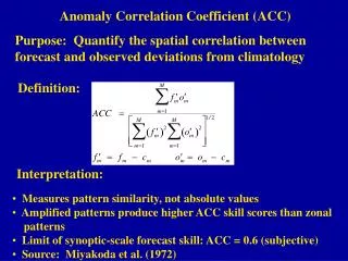
Technically… • r = covariation of X & Y / sd of X * sd of Y • Looks like this • But we won’t test you on the formula.
Pearson’s r is + when dv & iv increase together is – when dv & iv inversely related = 1 when vars perfectly + correlated = 0 when no correlation = -1 when vars perfectly – correlated Look at perfection. Properties of the correlation coefficient Perfect Correlation
Interpretation of correlation coefficient • To interpret r, we usually square it, so we have r2, which varies between 0 and 1 (no negative values). • r2 is the percentage of the variation of one variable explained the other variable. • Usually, we’re thinking of independent and dependent variables, so it becomes the % of variance in the dv explained by the iv.
Interpretation of correlation coef (cont.) • What we would like to have, of course, is a high r2. • But, don’t expect really high r2 values. • We rarely—even with several variables—explain 70, 80, 90% of the variance. (Causal relationships are complex.) • On the other hand, we try to find relationships in which the variables are more than minimally related.
Correlation coefficient (cont.) Remember: the correlation measures linear relationships
Correlation coefficient (cont.) • How do we get correlation output (from SPSS)? • Analyze-Correlate-Bivariate Option (you control): Pairwise or listwise deletion (will explain below). • Often one produces more than one correlation at a time (a correlation matrix)
Correlation coefficient (cont.) Looking at output makes these points clearer
Correlation coefficient (cont.) • Points to note on SPSS output (and to remember in general): • The table is symmetric; redundant information. • n’s for each variable may be larger than n’s on which the correlation is based. It’s easy to miss this; you shouldn’t. Listwise or pairwise deletion Look at next slide
Correlation coefficient (cont.) • The notion of significance levels applies equally well to r’s as to other statistics that we calculate. You won’t be tested on the formula. With r’s, you decide whether it’s a one- or two-tailed test (see above output). • Positive/negative direction depends on coding of variables—just as with cross-tabs.
Correlation coefficient (cont.) Direction of a positive relationship in a table Direction of a positive relationship in a figure
Correlation coefficient (cont.) • Saving grace: • Positive (conceptually) always mean “as one variable increases, so does the other variable.” • Negative always means “as one variable increases, the other variable decreases. • You do need to remember this “saving grace” and you need to pay attention to how variables are scored.
Correlation coefficient (cont.) • Can it be used with ordinal measures? • No, if one means strictly speaking, as it is not consistent with the underlying assumptions. • Yes, if one means will SPSS do the calculation. (SPSS is dumb that way.) • Yes, sometimes, if one means do people do it.
Correlation coefficient (cont.) • What do we think you should do? • Use of r’s is better justified if: One does have interval data. One has equal-appearing intervals (e.g., with thermometers; seven- point scales).
Correlation coefficient (cont.) • Is there any rule of thumb about what constitutes a low/med/high correlation? • No. Partly because the size of r’s depends on what kind of data one has. With individual data, r’s tend to be on the low end. With aggregate data for the same variables, r’s tend to be higher.
Correlation coefficient (cont.) • Cautionary notes Correlation ≠ causation. (No different from other measures of association.) There can be high correlation but no practical use and low correlation but great practical use. Example of the former: Family characteristics & success in school?
Correlation coefficient (cont.) • Cautionary notes (cont.) Beware of the ecological fallacy— making inferences about individuals based on data about aggregate units. Example: Precinct data may show a strong r between race and turnout, sug- gesting (to the not-very-careful) that one racial group votes at a much lower rate. Yet individual-level data may show that no such relationship exists.
Correlation coefficient (cont.) • Finally, an interesting example of r’s yielding useful information: In the 2000 election, r = .85 for # of times Gore and Bush visited various states. r = .50 for # of times Gore and Nader visited various states. What do you conclude from this?