Correlation Coefficient with Technology
Material Taken From: Mathematics for the international student Mathematical Studies SL Mal Coad , Glen Whiffen , John Owen, Robert Haese , Sandra Haese and Mark Bruce Haese and Haese Publications, 2004. Section 18B – Measuring Correlation. Correlation Coefficient with Technology. TI 84.

Correlation Coefficient with Technology
E N D
Presentation Transcript
Material Taken From:Mathematicsfor the international student Mathematical Studies SLMal Coad, Glen Whiffen, John Owen, Robert Haese, Sandra Haese and Mark BruceHaese and Haese Publications, 2004
Section 18B – Measuring Correlation Correlation Coefficient with Technology TI 84 Autograph Open a 2D Graph Page Data > Enter XY Data Set Enter your data Select Show Statistics Click OK Click Transfer to Results Box View > Results Box • Turn on the Diagnostics • Enter the data in L1 and L2 • LinReg L1, L2
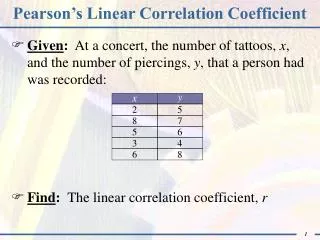
Example 1 At a father-son camp, the heights of the fathers and their sons were measured. Draw a scatter plot of the data. Calculate r Describe the correlation between the variables.
Example 2 The Botanical Gardens have been trying out a new chemical to control the number of beetles infesting their plants. The results are shown. Calculate r Describe the correlation between the variables.
Section 18A – Line of Best Fit (By Eye) At a tournament, athletes throw a discus. The age and distance thrown are recorded for each athlete:
Drawing the Line of Best Fit • Calculate mean of x values , and mean of y values • Mark the mean point on the scatter plot • Draw a line through the mean point that is through the middle of the data • equal number of points above and below line
Example 3 On a hot day, six cars were left in the sun for various lengths of time. The length of time each car was left in the sun was recorded, as well as the temperature inside the car at the end of the period. • Calculate and • Draw a scatter plot for the data • Plot the mean point and draw a line of best fit • Predict the temperature of a car which has been left in the sun for: • 35 minutes • 75 minutes • Comment on the reliability of your predictions
Section 18C – Linear Regression Scatter Plot Find a linear equation that best-fits the data.
Best Fit vs. Regression The problem with drawing a line of best fit by eye is that the line will vary from one person to the other.
Least Squares Regression Line • Consider the set of points below. • Square the distances and find their sum. • we want that sum to be small.
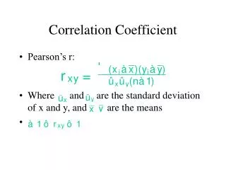
Least Squares Regression Formula Note:sxywill be given on an exam, while sx is found with the TI 84.
Example 4 Consider the data given: a) Given sxy ≈ -14.286, find the equation of the least squares regression line. b) Estimate the value of y when x = 6. Comment on the reliability of your estimate.
Some things to note: • The regression line is used for prediction purposes. • The regression line is less reliable when extended far beyond the region of the data.
Example 5 The table shows the sales for Hancock’s Electronics established in late 1998. Draw a scatterplot to illustrate this data. Given thatsxy≈ 12.5 find the correlation coefficient, r. Find the equation of the regression line, using the formula. Predict the sales figures for the year 2006, giving your answer to the nearest $10,000. Comment on the reasonableness of this prediction.
Regression Line with Technology TI 84 Autograph Open a 2D Graph Page Data > Enter XY Data Set Enter your data Select Show Statistics Click OK Click Transfer to Results Box View > Results Box • LinReg(ax +b) L1, L2 • where L1 contains your independent data. • and L2 contains your dependent data
Example 6 The table shows the annual income and average weekly grocery bill for a selection of families Construct a scatter plot to illustrate the data. Use technology to find the line of best fit. Estimate the weekly grocery bill for a family with an annual income of £95000. Comment on whether this estimate is likely to be reliable.
Homework • Complete Worksheet 2 • Pg 590 #6,7,8