Download
1 / 31
310 likes | 331 Views
This comparison study examines the fluxes (latent heat, sensible heat, stress) in the SW Indian and SW Pacific during summer and winter from 1997-2004. The data includes ocean reference experiment data, satellite and NCEP reanalysis data, and global wave data.

E N D
Flux Model Comparisons Note: There is a lot of detail slides that will be skipped.
Summer Winter SW Indian SW Indian SW Indian SW Pacific SW Pacific SW Pacific Drake Pass Drake Pass Drake Pass Cold Tongue Cold Tongue Cold Tongue Kuroshio Kuroshio Kuroshio Gulf Stream Gulf Stream Gulf Stream Global Global Global Modeled Mean of Fluxes (1997-2004) Latent Heat Flux (W m-2) W m-2 Sensible Heat Flux (W m-2) W m-2 Stress (N m-2) N m-2
Datasets (January 30, 1997 → December 31, 2004) • Coordinated Ocean Reference Experiment (CORE) version 1: • Combined satellite and NCEP reanalysis data. • 10 m Air Temperature, 10 m winds, 10 m specific humidity, and SLP. • Provided at 4 Times/Day • dx=1.875°, dy~1.875° • Reynolds (2006) OI SST: • Enhanced with Pathfinder AVHRR Data • Provided Daily • dx=0.25°, dy=0.25°; re-gridded to 1.875°. • NOAA Wavewatch 3 (NWW3) Modeled Global Wave Data (Tolman, 2002): • Utilizing the following data types: significant wave height (m), dominant wave period (s), and wave direction (degrees). • Provided 6 Times/Day • dx=1.25°, dy=1°; re-gridded to 1.875°
U(z)→wind at height z ϕ→stability parameter z0→ roughness length κ=0.4 → von Karman constant z =10 m → reference height L→ Monin-Obukhov stability length Estimating Stress • Two commonly applied approaches are: • with a drag coefficient (CD) and wind speed (U): • with a roughness length, z0, solve the log wind equation for u*:
Effect of Stability on Transfer Coefficients • This particular example is using the stress parameterization of Smith (1988). • Lines are isopleths of Tair-Tskin Heat Transfer Coeff. vs. Wind Speed Drag Coefficient vs. Wind Speed Unstable Unstable CD (x10-4) CH (x10-4) Stable Stable U10(m/s) U10(m/s)
Kuroshio Gulf Stream Drake Passage Other WBCs Near-Neutral Rib Stability (1997-2004) ~70% Near-Neutral 24.4 % Moderately Unstable * Expressed as a percentage of the ‘Local’ Rib distribution.
Atmospheric Stability Parameterizations • “Neutral Assumption”: • Stability functions for momentum, temperature, and moisture are set to zero. • “Old”: Businger-Dyer relations • Stable stratification (Businger et al. 1971 and Dyer 1974): • linear relationship • Unstable stratification (Businger 1966 and Dyer 1967): • non-linear relationship (more complex than previous) • “New”: (more recent and complex than Businger-Dyer) • Stable stratification (Beljaars and Holtslag 1991): • non-linear relationship • Unstable stratification (Benoit 1977): • modified and more complex form of Businger-Dyer
Sea-state Independent Parameterizations • Large and Pond (1981): • Neutral Drag coefficient: • Discontinuous at 10 m s-1 • Produces a neutral stress (i.e. stability has no impact on stress) • Large et al. (1994): • Neutral Drag coefficient: • Difference from Large and Pond: • Continuous at all wind speeds • Smith (1988): • Charnock (1955) based roughness length, α=0.011. • Dependent upon changes in u* • Differences from previous: • Stress is determined by roughness • Stress is influenced by stability
Sea-state Dependent Parameterizations • HEXOS (Smith et al. 1992, 1996) • Similar to Smith (1988), but roughness is now a function of inverse wave age (Cp/u*)-1: • Generally produces • Greater stress for rising seas (steeper waves), • Smaller stress for falling seas (swell). • Doesn’t apply for swell. • Taylor and Yelland (2001) • An alternative to HEXOS, where roughness length is a function of wave height (Hs) and wave-slope (Hs/L). • Differences from HEXOS: • No dependency on friction velocity. • Open-ocean wind stresses are less likely to be overestimated. • Bourassa (2006): • Adds a surface component to the log-wind profile, Uorb= π(Hs/Tp) • Shear is decreased when swell and wind are directionally aligned (i.e. a majority of cases). • Shear is increased when swell and wind are directionally opposed (i.e. outflow boundaries and fast-moving cold fronts). • Enhanced shear produces higher stresses, which is further enhanced by a Charnock-based roughness length, with an empirically derived Charnock parameter, α=0.035.
Observed (x) and Modeled (y) Friction Velocity (u*) 1.2 1.0 0.8 0.6 0.4 0.2 0.0 1.2 1.0 0.8 0.6 0.4 0.2 0.0 Smith (1988) Large and Pond (1981) 0.0 0.2 0.4 0.6 0.8 1.0 1.2 0.0 0.2 0.4 0.6 0.8 1.0 1.2 1.2 1.0 0.8 0.6 0.4 0.2 0.0 1.2 1.0 0.8 0.6 0.4 0.2 0.0 Bourassa (2006) Taylor and Yelland (2001) 0.0 0.2 0.4 0.6 0.8 1.0 1.2 0.0 0.2 0.4 0.6 0.8 1.0 1.2
Results of Bourassa (2006) Compared to SWS2 Observations • This variation has a non-zero Newtonian frame of references and displacement height. • Displacement height is a fraction of the significant wave height. • Charnock’s constant is actually constant.
Wildly Different Models & Observations • Courtesy Will Drennan
Consistency Check • An eighteen member ensemble of flux ‘models’ is used to check for consistency. • Six drag coefficient or roughness length parameterizations • Three stability parameterizations (including neutral stability) • Results in eighteen (six times three) combinations • Extremes at the high and low ends are inconsistent. • This consistency check focuses on more typical values • The inter-quartile range (IQR) is calculated for each grid cell for each season and each flux model • The diagnostic we use for consistency is the standard deviation of the IQR • Note that this diagnostic focuses more on a difference in range of values than in a shift of the mean.
Latent Heat Flux Inconsistencies Standard Deviation from Mean IQR (1997-2004)
Stress Inconsistencies Standard Deviation from Mean IQR (1997-2004)
Stand-Alone Flux Algorithms • COAREv3.0 (Fairall et al. 2003): Most state-of-the-art flux algorithm to date. • Many additional considerations, but only the following are utilized: • Taylor and Yelland (2001) Roughness Length. • Businger-Dyer Relations blended with Grachev et al. (2000) for Unstable conditions. • Beljaars and Holtslag (1991) for Stable conditions. • Rib to reduce # of iterations for stability down to 3 (previous version required 20). • Webb et al. (1980) correction to improve the accuracy of Latent Heat Flux estimates. • A more up-to-date temperature and moisture roughness length parameterization, relative to what is utilized by the previous stress-related parameterizations. • Kara et al. (2005): A Polynomial Curve Fit to COAREv3.0. • 0 Stability iterations. • No sea-state dependency. • Polynomial expressions are supplemented by a look-up table to calculate heat, moisture, and momentum transfer coefficients. • Stability and wind speed variations are implicitly accounted for. • Advertises reasonable agreement with COAREv3.0 at 5X greater efficiency.
Stress-Related Comparison • Examined at the Gulf Stream and Drake Passage. • Stability parameterizations held constant, allowing for direct comparison of stress-related parameterizations. • Only results from the ‘New’ stability parameterizations are shown. Results from remaining parameterizations are qualitatively similar. • A seasonal comparison is included: Summer vs. Winter. • Seasons are hemisphere-relative. • Key Features to Notice: • The tails of the distributions are the episodic events. • Distinctions between sea state independent-dependent parameterizations. • Seasonal changes in the strength of episodic events, as determined by the estimated flux magnitudes. • Seasonal changes in parameterized consistency.
Summer: July - September Winter: January - March Moderate Intense Extreme! RMS Diff. from Mean: ≤ 5% 3.70 % ≤ 5 W m-2 10.09 % Gulf Stream: Latent Heat Flux RMS Diff. from Mean: ≤ 5% 9.21 % ≤ 5 W m-2 19.13 % ← Fractional → ← Absolute → Gulf Stream Region: IQR Inconsistencies
Summer: January - March Winter: July - September Moderate Intense Extreme! RMS Diff. from Mean: ≤ 5% 8.42 % ≤ 5 W m-2 74.03 % RMS Diff. from Mean: ≤ 5% 7.59 % ≤ 5 W m-2 58.80 % ← Fractional → ← Absolute → Drake Passage: IQRInconsistencies Drake Passage: Latent Heat Flux
Summer: July - September Winter: January - March Moderate Intense Extreme! RMS Diff. from Mean: ≤ 5% 4.02 % ≤ 5 W m-2 76.34 % RMS Diff. from Mean: ≤ 5% 3.56 % ≤ 5 W m-2 28.24 % ← Fractional → ← Absolute → Gulf Stream Region: IQRInconsistencies Gulf Stream: Sensible Heat Flux
Summer: January - March Winter: July - September Moderate Intense Extreme! RMS Diff. from Mean: ≤ 5% 10.79 % ≤ 5 W m-2 46.64 % RMS Diff. from Mean: ≤ 5% 8.46 % ≤ 5 W m-2 65.49 % ← Fractional → ← Absolute → Drake Passage: IQRInconsistencies Drake Passage: Sensible Heat Flux
Summer: July - September Winter: January - March Moderate Intense Extreme! RMS Diff. from Mean: ≤ 5% 4.02 % ≤ .05 N m-2 97.28 % RMS Diff. from Mean: ≤ 5% 0.89 % ≤ .05 N m-2 71.95 % ← Fractional → ← Absolute → Gulf Stream Region: IQRInconsistencies Gulf Stream: Stress
Summer: January - March Winter: July - September Moderate Intense Extreme! RMS Diff. from Mean: ≤ 5% 2.58 % ≤ .05 N m-2 83.17 % RMS Diff. from Mean: ≤ 5% 1.72 % ≤ .05 N m-2 73.20 % ← Fractional → ← Absolute → Drake Passage: IQRInconsistencies Drake Passage: Stress
Summer: July - September Winter: January - March Moderate Intense Extreme! RMS Diff. from Mean: ≤ 5% 0.36 % ≤ 5x10⁻⁸ N m-3 35.58 % RMS Diff. from Mean: ≤ 5% 1.60 % ≤ 5x10⁻⁸ N m-3 74.87 % ← Fractional → ← Absolute → Gulf Stream Region: IQRInconsistencies Gulf Stream: Curl of the Stress
Summer: January - March Winter: July - September Moderate Intense Extreme! RMS Diff. from Mean: ≤ 5% 0.46 % ≤ 5x10⁻⁸ N m-3 31.52 % RMS Diff. from Mean: ≤ 5% 0.59 % ≤ 5x10⁻⁸ N m-3 42.61 % ← Fractional → ← Absolute → Drake Passage: IQRInconsistencies Drake Passage: Curl of the Stress
Result Summary • Parameterization consistency tends to deteriorate in response to the strength of the forcing. • There is relatively large amount of strong forcing in high latitudes • More common in the Southern Ocean • Stronger events in the NH mid to high latitudes • Inconsistencies are ‘primarily’ due to various sea-state dependencies. • More pronounced in the Gulf Stream than in Drake Passage. • Indicates that sea-state in Drake Passage is more swell dominant, where the Gulf Stream is more wind-wave dominant. • Wind-waves provide greater roughness than swell, which translates to greater stress and heat flux estimates. • Non-neutral stability provides relatively ‘minor’ inconsistencies with regard to the COAREv3 and Kara et al. (2005) algorithms.
Conclusions • How Practical Is the Assumption of Sea-state Independence? • Depends on the region . • Tropical, open-ocean regions (i.e. where episodic wind-stress and wind-waves are minimal) provide the best consistency. • WBC and ice-edge regions contain a higher probability of episodically induced wind stress and sea-state conditions, where associated inconsistencies are physically significant. • Depends on the time of year. • Summer months contain relatively mild episodic events over most regions (exception: tropical storms and monsoons). • Winter months are prone to fast moving cold-air outbreaks, which result in substantially younger seas with higher wind-wave heights, contributing to higher roughness lengths, which finally produces greater heat flux and stress estimates. Consistency diminishes as flux magnitude increases.
Conclusions - Continued • How Good is the Assumption of Neutral Stratification? • Depends on the region. • Higher wind speeds result in a higher probability of ‘near-neutral’ events, which is why open-ocean regions (i.e. Southern Oceans) tend to be dominated by ‘near-neutral’ events. • Cold-air outbreaks are fairly common in WBC and ice edge regions, resulting in highly unstable conditions, due to the contrast of warm SSTs with a cold and dry air mass. • Depends on the flux diagnostic being examined. • Latent and Sensible heat fluxes are the Most sensitive to changes in atmospheric stability, and therefore the estimates are most adversely affected by non-neutral conditions. • If a modeler is mainly concerned with estimating stress, he/she could use the ‘Neutral’ assumption for a greater variety of atmospheric conditions.
References • Beljaars, A. C. M., and A. A. M. Holtslag, 1991: Flux parameterization over land surfaces for atmospheric models, J. Appl. Meteor.,30, 327-341. • Benoit, R., 1977: On the integral of the surface layer profile-gradient functions. J. Appl. Meteor., 16, 859-560. • Bourassa, M. A., 2006: Satellite-based observations of surface turbulent stress during severe weather, Atmosphere - ocean interactions, Vol. 2., W. Perrie, Ed., Wessex Institute of Technology Press, 35 – 52 pp. • Businger, J. A., 1966: Transfer of heat and momentum in the atmospheric boundary layer. Proc. Arctic Heat Budget and Atmospheric Circulation, Santa Monica, CA, RAND Corporation, 305-332. • ______, J. C. Wyngaard, Y. Izumi, and E. F. Bradley, 1971: Flux profile relationships in the atmospheric surface layer. J. Atmos. Sci., 28, 181-189. • Charnock, H., 1955: Wind stress on a water surface. Quart. J. Roy. Meteor. Soc., 81, 639-640. • Dyer, A. J., 1967: The turbulent transport of heat and water vapour in an unstable atmosphere. Quart. J. Roy. Meteor. Soc., 93, 501-508. • ______, 1974: A review of flux-profile relationships. Bound.-Layer Meteor., 7, 363-372. • Fairall, C. W., E. F. Bradley, J. E. Hare, A. A. Grachev, and J. B. Edson, 2003: Bulk parameterizations of air-sea fluxes: updates and verification for the COARE algorithm. J. Climate., 16, 571-591. • Kara, A. B., H. E. Hurlburt, and A. J. Wallcraft, 2005: Stability-dependent exchange coefficients for air-sea fluxes. J. Atmos. and Oceanic Technol., 22, 1080-1094. • Large, W. G., and S. Pond, 1981: Open ocean momentum flux measurements in moderate to strong winds. J. Phys. Oceanogr., 11, 324-336. • ______, J. C. McWilliams, and S. C. Doney, 1994: Oceanic vertical mixing: a review and a model with a nonlocal boundary layer parameterization. Rev. Geophys.,32. 363-403. • ______, and S. G. Yeager, 2004: Diurnal to decadal global forcing for ocean and sea-ice models: The data sets and flux climatologies. NCAR Technical Note, NCAR/TN-460†STR, 105pp. • Reynolds, R. W., 2006: Personal communication. • Smith, S. D., 1988: Coefficients for sea surface wind stress, heat flux, and wind profiles as a function of wind speed and temperature. J. Geophys. Res.,93, 15,467-15,472. • ______, R. J. Anderson, W. A. Oost, C. Kraan, N. Maat, J. DeCosmo, K. B. Katsaros, K. L. Davidson, K. Bumke, L. Hasse, and H. M. Chadwick, 1992: Sea surface wind stress and drag coefficients: the HEXOS results. Bound.-Layer. Meteoro., 60, 109-142. • Taylor, P. K., and M. J. Yelland, 2001: The Dependence of sea surface roughness on the height and steepness of the waves. J. Phys. Oceanogr., 31, 572-590. • Tolman, H. L., 2002: Validation of WAVEWATCH III version 1.15 for a global domain. Technical Note. Environmental Modeling Center, Ocean Modeling Branch, NOAA.
Atmospheric Stability Parameterizations • “Neutral Assumption”: • Stability parameters for momentum, temperature, and moisture are set to zero. • “Old”: Businger-Dyer relations • stable stratification (Businger et al. 1971 and Dyer 1974): • unstable stratification (Businger 1966 and Dyer 1967): • “New”: • stable stratification (Beljaars and Holtslag 1991): • unstable stratification (Benoit 1977): ϕm-> stability parameter for momentum ϕt-> stability parameter for temperature and moisture L -> Monin-Obukhov Stability Length am= 0.7, bm= 0.75, c = 5.0, d = 0.35 at,q= 1.0, bt,q= 0.667