Download
1 / 60
610 likes | 793 Views
Explore the world of climate modeling with insights on climate vs. weather, atmospheric modeling strategies, and parameterization techniques. Learn from real NCAR scientists about climate change impacts, numerical weather prediction, and the conceptual framework for climate modeling. Discover the intricate processes and physical parameterizations involved, from grid discretizations to model solutions.

E N D
An Introduction to Climate Modeling Andrew Gettelman National Center for Atmospheric Research Boulder, Colorado USA Assistance from: J. J. Hack (NCAR)
Simulate the future on your desktop Climate Modeling Science, Statistics, Parameterization, Results It’s all in here! A. Gettelman& J. Hack Real NCAR Scientists
Outline • What is Climate • Why is climate different from weather and forecasting • Hierarchy of atmospheric modeling strategies • Focus on 3D General Circulation models (GCMs) • Conceptual Framework for General Circulation Models • Parameterization of physical processes • concept of resolvable and unresolvable scales of motion • approaches rooted in budgets of conserved variables • Model Validation and Model Solutions
Question 1: What is Climate? • Average/Expected ‘Weather’ • The temperature & precipitation range • Distribution of all possible weather • Record of Extreme events
Climate change and its manifestation in terms of weather (climate extremes) (1) What is Climate?
Climate change and its manifestation in terms of weather (climate extremes)
Climate change and its manifestation in terms of weather (climate extremes)
Impacts of Climate Change (- +) Observed Change 1950-1997 Snowpack Temperature (-+) Mote et al 2005
Observed Temperature Records IPCC, 3rd Assessment, Summary For Policymakers
‘Anthropogenic’ Changes Radiative Forcing (Wm-2) 1000 1200 1400 1600 1800 2000
560ppmv CO2 ~2060 ‘Anthropogenic’ Changes (2)
Question 2 • What is the difference between Numerical Weather Prediction and Climate prediction?
Climate v. Numerical Weather Prediction • NWP: • Initial state is CRITICAL • Don’t really care about whole PDF, just probable phase space • Non-conservation of mass/energy to match observed state • Climate • Get rid of any dependence on initial state • Conservation of mass & energy critical • Want to know the PDF of all possible states • Don’t really care where we are on the PDF • Really want to know tails (extreme events)
Question 3 How can we predict Climate (50 yrs) if we can’t predict Weather (10 days)? Statistics!
Conceptual Framework for Modeling • Can’t resolve all scales, so have to represent them • Energy Balance / Reduced Models • Mean State of the System • Energy Budget, conservation, Radiative transfer • Dynamical Models • Finite element representation of system • Fluid Dynamics on a rotating sphere • Basic equations of motion • Advection of mass, trace species • Physical Parameterizations for moving energy • Scales: Cloud Resolving/Mesoscale/Regional/Global • Global= General Circulation Models (GCM’s)
Earth System Model ‘Evolution’ 2000 2005
Modeling the Atmospheric General Circulation Requires understanding of : • atmospheric predictability/basic fluid dynamics • physics/dynamics of phase change • radiative transfer (aerosols, chemical constituents, etc.) • interactions between the atmosphere and ocean (El Nino, etc.) • solar physics (solar-terrestrial interactions, solar dynamics, etc.) • impacts of anthropogenic and other biological activity Basic Process: • iterate finite element versions of dynamics on a rotating sphere • Incorporate representation of physical processes
Meteorological Primitive Equations • Applicable to wide scale of motions; > 1hour, >100km
Global Climate Model Physics Terms F, Q, and Sq represent physical processes • Equations of motion, F • turbulent transport, generation, and dissipation of momentum • Thermodynamic energy equation, Q • convective-scale transport of heat • convective-scale sources/sinks of heat (phase change) • radiative sources/sinks of heat • Water vapor mass continuity equation • convective-scale transport of water substance • convective-scale water sources/sinks (phase change)
Grid Discretizations Equations are distributed on a sphere • Different grid approaches: • Rectilinear (lat-lon) • Reduced grids • ‘equal area grids’: icosahedral, cubed sphere • Spectral transforms • Different numerical methods for solution: • Spectral Transforms • Finite element • Lagrangian (semi-lagrangian) • Vertical Discretization • Terrain following (sigma) • Pressure • Isentropic • Hybrid Sigma-pressure (most common)
Model Physical Parameterizations Physical processes breakdown: • Moist Processes • Moist convection, shallow convection, large scale condensation • Radiation and Clouds • Cloud parameterization, radiation • Surface Fluxes • Fluxes from land, ocean and sea ice (from data or models) • Turbulent mixing • Planetary boundary layer parameterization, vertical diffusion, gravity wave drag
Basic Logic in a GCM (Time-step Loop) For a grid of atmospheric columns: • ‘Dynamics’: Iterate Basic Equations Horizontal momentum, Thermodynamic energy, Mass conservation, Hydrostatic equilibrium, Water vapor mass conservation • Transport ‘constituents’ (water vapor, aerosol, etc) • Calculate forcing terms (“Physics”) for each column Clouds & Precipitation, Radiation, etc • Update dynamics fields with physics forcings • Gravity Waves, Diffusion (fastest last) • Next time step (repeat)
Physical Parameterization To close the governing equations, it is necessary to incorporate the effects of physical processes that occur on scales below the numerical truncation limit • Physical parameterization • express unresolved physical processes in terms of resolved processes • generally empirical techniques • Examples of parameterized physics • dry and moist convection • cloud amount/cloud optical properties • radiative transfer • planetary boundary layer transports • surface energy exchanges • horizontal and vertical dissipation processes • ...
F F Sq Sq Q
Atmospheric Energy Transport Synoptic-scale mechanisms • hurricanes • extratropical storms http://www.earth.nasa.gov
Process Models and Parameterization • Boundary Layer • Clouds • Stratiform • Convective • Microphysics
Other Energy Budget Impacts From Clouds http://www.earth.nasa.gov
Energy Budget Impacts of Atmospheric Aerosol http://www.earth.nasa.gov
Scales of Atmospheric Motions/Processes Resolved Scales Global Models Future Global Models Cloud/Mesoscale/Turbulence Models Cloud Drops Microphysics CHEMISTRY Anthes et al. (1975)
Examples of Global Model Resolution ~300km 50-100km Typical Climate Application Next Generation Climate Applications
High Resolution Art Global Model Simulation 100km x 100km Global Model Precipitation NCAR CCM3 run on Earth Simulator, Japan
Key Uncertainties for Climate (1): • Low Clouds over the ocean: Reflect Sunlight (cool) : Dominant Effect Trap heat (warm) More Clouds=Cooling Fewer Clouds=Warming
Parameterization of Clouds Cloud amount (fraction) as simulated by 25 atmospheric GCMs Weare and Mokhov (1995)
Low Clouds Over the Ocean Change in low cloud with 2xCO2 2 Models: Changes are OPPOSITE!
Key Uncertainties for Climate (2): 2. High Clouds: Dominant effect is that they Trap heat (warm) More Clouds=Warming Fewer Clouds=Cooling
Key Uncertainties for Climate (3): • Water Vapor: largest greenhouse gas Increasing Temp=Increasing water Vapor (more greenhouse) Effect is expected to ‘amplify’ warming through a ‘feedback’ 1D Radiative-Convective Model: Higher humidity=>warmer surface
Summary • Global Climate Modeling • complex and evolving scientific problem • parameterization of physical processes pacing progress • observational limitations pacing process understanding • Parameterization of physical processes • opportunities to explore alternative formulations • exploit higher-order statistical relationships? • exploration of scale interactions using modeling and observation • high-resolution process modeling to supplement observations • e.g., identify optimal truncation strategies for capturing major scale interactions • better characterize statistical relationships between resolved and unresolved scales
How can we evaluate simulation quality? • Compare long term mean climatology • average mass, energy, and momentum balances • tells you where the physical approximations take you • but you don’t necessarily know how you get there! • Consider dominant modes of variability • provides the opportunity to evaluate climate sensitivity • response of the climate system to a specific forcing factor • exploit natural forcing factors to test model response • diurnal and seasonal cycles, El Niño Southern Oscillation (ENSO), solar variability
Comparison of Mean Simulation Properties 1 Simulated Precipitation Observed Precipitation
Comparison of Mean Simulation Properties 1 Simulated Precipitation Difference: Sim- Observed
Comparison of Mean Simulation Properties 2 Simulated Land Temp Observed Land Temp
Comparison of Mean Simulation Properties 2 Simulated Land Temp Difference: Sim- Observed
Testing AGCM Sensitivity Cloud (OLR) Anomalies and ENSO Observed Simulated Hack (1998) More Cloud Less Cloud
Turning The Crank: Results • Simulations of Atmospheric Model Coupled to Ocean • Present Day Climate • Simulations into the future with ‘Scenarios’ • Different Models=Different ‘Sensitivity’ • Potential Changes in Temp, Precip
Observations: 20th Century Warming Model Solutions with Human Forcing