Download
1 / 30
300 likes | 418 Views
Introduction to basic two-level regression modeling, examining cross-national data structures in sociology and political sciences. Discusses the importance of analyzing individual and country-level characteristics to explain variability.

E N D
Two introductory points: 1. Hierarchical cross-national data structures arecommon within the field of sociology and political sciences, and ESS is a good example of such structures. Hierarchical cross-national data structures mean that we have information on the level of individuals and on the level of countries. The problem is how to explain one individual-level characteristic (variable) using both (a) other individual-level characteristics (variables), and (b) country-level characteristics (variables).
. 2. The old solution is to pool data from all countries and use country-level characteristics assigned to individuals as all other individual characteristics. There are three consequences of this (cross-sectional pooling) strategy: (a) For effects of individual-level variables we increase N so that these effects become significant while in the reality they might be not significant. (b) For effects of country-level variables we also increase N so that these effects become significant while in the reality they might be not significant. [Both (a) and (b) lead to increasing the probability of “false positive” = Error Type I, the error of rejecting a "correct" null hypothesis]. (c) Case dependency. Units of analysis are not independent – what is required by regular regression.
. Ignoring the statistical significance, for effects of individual-level variables, a pooling strategy can only be successful if countries are homogeneous. The extent that this condition really is met is indicated by the intra-class correlation. Usually this condition is poorly met. .
The basic two-level regression model with a continuous outcome An example taken from Stefan Dahlberg, Department of Political Science, Goteborg University (2007) We have opinion survey data from J countries with a number of respondents, i.e. voters i, ni, in each country j. On the individual level we have an outcome variable (Y) measured as the absolute distance between a voters self-placement on a left-right scale and the position, as ascribed by the voter, for the party voted for on the same scale. This dependent variable is called “proximity.” .
Two-levels We have two independent variables: X - education, and Z - the degree of proportionality of the electoral system. We assume that more educated people tend to vote consistently (high proximity). More proportional systems are expected to induce proximity voting since voters tend to view the elections as an expression of preferences rather than a process of selecting government. We have three variables on two different levels: Y proximity, X education (individual level) Z proportionality (country-level). .
Eq. 1 The simplest way to analyze the data is to make separate regressions in each country such as: (1.1.) Yij = α0j + β1jXij + eij The difference compared to a more ordinary regression model is that we assume that intercepts and slopes are varying between electoral systems, i.e. each country has its own intercept and slope, denoted by α0j and β1j. .
Interpretation The error term, eij is expected to have a mean of zero and a variance to be estimated. Since the intercept and slope coefficients are assumed to vary across countries they are often referred to as random coefficients. Across all countries the regression coefficients βj have a distribution with some mean and variance. .
Eq. 2-3 The next step in the hierarchical regression analysis is to introduce the country-level explanatory variable proportionality in an attempt to explain the variation of the regression coefficients α0j and β1j. (1.2) α0j = γ00 + γ01Zj + u0j and (1.3)β1j = γ10 + γ11Zj + u1j .
Interpretation Equation 1.2 predicts the average degree of proximity voting in a country (the intercept α0j ) by the degree of proportionality in the electoral system (Z). Equation 1.3 denotes that the relationship, as expressed by the coefficient β1jbetween proximity voting (Y) and level of education (X), is depending on the degree of proportionality within the electoral system (Z). The degree of proportionality is here functioning as an interactive variable where the relationship between proximity voting and education varies according to the values on the second level variable proportionality.
. The u-terms u0j and u1j in equation 1.2 and 1.3 are random residual error terms at the country level. The residual errors uj are assumed to have a mean of zero and to be independent from the residual errors eij at the individual level. The variance of the residual errors u0j is specified as σ2u0 and the variance of the residual errors u1j is specified as σ2u1.
. In equation 1.2 and 1.3 the regression coefficients γ are not assumed to vary across countries since they have the denotation j in order to indicate to which country they belong. As they apply to all countries the coefficients are referred to as fixed effects. All the between-country variation left in the β coefficients, after predicting these with the country variable proportionality (Zj), is then assumed to be the residual error variation. This is captured by the error term uj, which are denoted with j to indicate which country it belongs to. .
Eq. 4 The equations 1.2 and 1.3 can then be substituted into equation 1.1 and by rearranging them we have: (1.4) Yij= γ00 + γ10Xij + γ01Zj + γ11XijZj + u1jXij + u0j + eij .
Interpretation In terms of variable labels the equation 1.4 states: proximityij = γ00 + γ10 educationij + γ01 proportionalityj + γ11 educationij * proportionalityj + u1j educationij + u0j + eij
. The first part of equation 1.4: γ00 + γ10Xij + γ01Zj + γ11XijZj is the fixed coefficients/effects. The term XijZj is an interaction term that is included in the model as a consequence of the modeling of the varying regression slope β1j on individual level variable Xij with the country level Zj.
. The last part of the equation 1.4 u1jXij + u0j + eij is a part of the random coefficients. The fact that the explanatory variable Xij is multiplied with the error term, u1jXij, the resulting total error will be different for different values of Xij.
. The error terms are heteroscedastic instead of homoscedastic as assumed in ordinary regression models where the residual errors are assumed to be independent of the values of the explanatory variable. [Random variables are heteroscedastic if they have different variances for the relevant subgrups. The complementary concept is called homoscedasticity. Note: The alternative spelling homo- or heteroskedasticity is equally correct and is also used frequently. The term means "differing variance" and comes from the Greek "hetero" (different) and "skedasis" (dispersion).]
. Dealing with the problem of heteroscedasticyis one of the main reasons for why multilevel models are preferable over regular OLS models when analyzing hierarchical nested data used.
SUMMING UP: Known in literature under a variety of names Hierarchical linear model (HLM) Random coefficient model Variance component model Multilevel model Contextual analysis Mixed linear model Mixed effects model Acknowldegements: Materials in the following are based on Prof. Joop J. Hox introductory lectures on HLM delivered at the 2011 QMSS2 Summer School in Leuven
Multi-level data structure Groups at different levels may have different sizes Response (outcome) variable at lowest level Explanatory variables at all levels The statistical model assumes sampling at all levels Ex: education family longitudinal level 3 schools classes level 2 classes families level 1 pupils members occasions (waves)
Problems with Hierarchical Data Structure I Assume DV (response) variable on lowest level(level 1). We want to predict this, using explanatoryvariables at all available levels - How? - What is the proper sample size? - What if relations are not the same in different groups? Traditional approaches: Disaggregate all variables to the lowest level Do standard analyses (anova, multiple regression) Aggregate all variables to the highest level Do standard analyses (anova, multiple regression) Ancova with groups as factor Some improvements: explanatory variables as deviations from their group mean have both deviation score & disaggregated group mean aspredictor (separates individual and group effects) What is wrong with this?
Problems with Hierarchical Data Structure II Multiple Regression assumes: independent observations independent error terms equal variances of errors for all observations(assumption of homoscedastic errors) normal distribution for errors With hierarchical data observations are not independent errors are not independent different observations may have errors with differentvariances (heteroscedastic errors)
Problems with Hierarchical Data Structure III Observations in the same group are generally notindependent - they tend to be more similar than observations from different groups - selection, shared history, contextual group effects The degree of similarity is indicated by the intraclasscorrelation rho: r Kish: roh (rate of homogeneity) Standard statistical tests are not at all robust againstviolation of the independence assumption
Graphical Pictureof 2-level regression Model School level Student level Outcome variable on pupil level - Explanatory variables at both levels: individual & group - Residual error at individual level - Plus residual error at school level School size error error Grade Student gender
Graphical Pictureof 2-level regression Model School level Student level Essential points: Explanatory variables characterize individuals and/or groups Average value of individual variables may differ across groups = most variables have both within-group and between-group variation Groups do make a difference: the effect of an individualexplanatory variable may be different in different groups School size error error Grade Student gender
Assumptions Yij= [g00+ g10Xij + g01Zj + g11ZjXij] + [u1jXij+ u0j+ eij] Individual level errors eij independent; normal distribution with mean zero and same variance se² in all groups Group level errors u.j independent; multivariate normal distribution with means zero and (co)variances su² in covariance matrix W (omega) Group level errors u.j independent from individual errors eij - plus usual assumptions of multiple regression analysis - linear relations, explanatory variables measured without error
Types of HLM Models Intercept-only Model Intercept only model (null model, baseline model) Contains only intercept and corresponding error terms At the lowest (individual) level we have Yij= b0j+ eij and at the second level b0j= g00+ u0j hence Yij= g00+ u0j+ eij Used to decompose the total variance and to compute theintraclass correlation r (rho) r = (group level variance / total variance) r = expected correlation between 2 individuals in same group
Fixed Model: Only fixed effects for level-1 explanatory variables: slopes are assumed not to vary across groups At the lowest (individual) level we have Yij = b0j+ b1jXij+ eij and at the second level b0j = g00+ u0j and b1j= g10 hence Yij= g00+ g10Xij+ u0j+ eij Intercepts vary across groups, slopes are the same Similar to ANCOVA with random grouping factor also called variance component model Fixed effects for level-2 explanatory variables added next
Random Coefficient Model Assumes intercept and slopes vary across groups Yij= b0j+ b1jXij+ eij and at the second level b0j= g00+ u0j and b1j= g10+ u1j hence Yij= g00+ g10Xij+ u1jXij+ u0j+ eij The full multilevel model adds interactions to model the slope variation
Full Multilevel Regression Model Explanatory variables at all levels Higher level variables predict variation of lowest level intercept and slopes At the lowest (individual) level we have Yij= b0j+ b1jXij+ eij and at the second level b0j= g00+ g01Zj+ u0j and b1j= g10+ g11Zj+ u1j hence Yij= g00+ g10Xij+ g01Zj+ g11ZjXij+ u1jXij+ u0j+ eij Predicting the intercept implies a direct effect Predicting slopes implies cross-level interactions