Download
1 / 30
330 likes | 458 Views
This guide explores the statistical methods for analyzing laboratory data, focusing on regression analysis for quantitative prediction. It discusses key assumptions such as linearity, independence, constant variance, and the normality of errors, which underpin the validity of statistical inferences. The consequences of violating these assumptions, such as heteroscedasticity and its impact on prediction accuracy, are examined. The document also highlights the importance of recording and replicating analyses and presents a fluorescein example to illustrate the relationship between intensity and concentration, which is crucial for calibration in laboratory settings.

E N D
Regression and Calibration SPH 247 Statistical Analysis of Laboratory Data SPH 247 Statistical Analysis of Laboratory Data
Quantitative Prediction • Regression analysis is the statistical name for the prediction of one quantitative variable (fasting blood glucose level) from another (body mass index) • Items of interest include whether there is in fact a relationship and what the expected change is in one variable when the other changes SPH 247 Statistical Analysis of Laboratory Data
Assumptions • Inference about whether there is a real relationship or not is dependent on a number of assumptions, many of which can be checked • When these assumptions are substantially incorrect, alterations in method can rescue the analysis • No assumption is ever exactly correct SPH 247 Statistical Analysis of Laboratory Data
Linearity • This is the most important assumption • If x is the predictor, and y is the response, then we assume that the average response for a given value of x is a linear function of x • E(y) = a + bx • y = a + bx + ε • ε is the error or variability SPH 247 Statistical Analysis of Laboratory Data
In general, it is important to get the model right, and the most important of these issues is that the mean function looks like it is specified • If a linear function does not fit, various types of curves can be used, but what is used should fit the data • Otherwise predictions are biased SPH 247 Statistical Analysis of Laboratory Data
Independence • It is assumed that different observations are statistically independent • If this is not the case inference and prediction can be completely wrong • There may appear to be a relationship even though there is not • Randomization and then controlling the treatment assignment prevents this in general SPH 247 Statistical Analysis of Laboratory Data
Note no relationship between x and y • These data were generated as follows: SPH 247 Statistical Analysis of Laboratory Data
Constant Variance • Constant variance, or homoscedacticity, means that the variability is the same in all parts of the prediction function • If this is not the case, the predictions may be on the average correct, but the uncertainties associated with the predictions will be wrong • Heteroscedacticity is non-constant variance SPH 247 Statistical Analysis of Laboratory Data
Consequences of Heteroscedacticity • Predictions may be unbiased (correct on the average) • Prediction uncertainties are not correct; too small sometimes, too large others • Inferences are incorrect (is there any relationship or is it random?) SPH 247 Statistical Analysis of Laboratory Data
Normality of Errors • Mostly this is not particularly important • Very large outliers can be problematic • Graphing data often helps • If in a gene expression array experiment, we do 40,000 regressions, graphical analysis is not possible • Significant relationships should be examined in detail SPH 247 Statistical Analysis of Laboratory Data
Statistical Lab Books • You should keep track of what things you try • The eventual analysis is best recorded in a file of commands so it can later be replicated • Plots should also be produced this way, at least in final form, and not done on the fly • Otherwise, when the paper comes back for review, you may not even be able to reproduce your own analysis SPH 247 Statistical Analysis of Laboratory Data
Fluorescein Example • Standard aqueous solutions of fluorescein (in pg/ml) are examined in a fluorescence spectrometer and the intensity (arbitrary units) is recorded • What is the relationship of intensity to concentration • Use later to infer concentration of labeled analyte SPH 247 Statistical Analysis of Laboratory Data
> fluor.lm <- lm(intensity ~ concentration) > summary(fluor.lm) Call: lm(formula = intensity ~ concentration) Residuals: 1 2 3 4 5 6 7 0.58214 -0.37857 -0.23929 -0.50000 0.33929 0.17857 0.01786 Coefficients: Estimate Std. Error t value Pr(>|t|) (Intercept) 1.5179 0.2949 5.146 0.00363 ** concentration 1.9304 0.0409 47.197 8.07e-08 *** --- Signif. codes: 0 `***' 0.001 `**' 0.01 `*' 0.05 `.' 0.1 ` ' 1 Residual standard error: 0.4328 on 5 degrees of freedom Multiple R-Squared: 0.9978, Adjusted R-squared: 0.9973 F-statistic: 2228 on 1 and 5 DF, p-value: 8.066e-08 SPH 247 Statistical Analysis of Laboratory Data
Use of the calibration curve SPH 247 Statistical Analysis of Laboratory Data
Measurement and Calibration • Essentially all things we measure are indirect • The thing we wish to measure produces an observed transduced value that is related to the quantity of interest but is not itself directly the quantity of interest • Calibration takes known quantities, observes the transduced values, and uses the inferred relationship to quantitate unknowns SPH 247 Statistical Analysis of Laboratory Data
Measurement Examples • Weight is observed via deflection of a spring (calibrated) • Concentration of an analyte in mass spec is observed through the electrical current integrated over a peak (possibly calibrated) • Gene expression is observed via fluorescence of a spot to which the analyte has bound (usually not calibrated) SPH 247 Statistical Analysis of Laboratory Data
Correlation • Wright peak-flow data set has two measures of peak expiratory flow rate for each of 17 patients in l/min. • ISwR library, data(wright) • Both are subject to measurement error • In ordinary regression, we assume the predictor is known • For two measures of the same thing with no error-free gold standard, one can use correlation to measure agreement SPH 247 Statistical Analysis of Laboratory Data
> setwd("c:/td/classes/SPH247 2013 Spring") > source(“wright.r”) > cor(wright) std.wrightmini.wright std.wright 1.0000000 0.9432794 mini.wright 0.9432794 1.0000000 > wplot1()-----------------------------------------------------File wright.r:library(ISwR) data(wright) attach(wright) wplot1 <- function() { plot(std.wright,mini.wright,xlab="Standard Flow Meter", ylab="Mini Flow Meter",lwd=2) title("Mini vs. Standard Peak Flow Meters") wright.lm <- lm(mini.wright ~ std.wright) abline(coef(wright.lm),col="red",lwd=2) } detach(wright) SPH 247 Statistical Analysis of Laboratory Data
Issues with Correlation • For any given relationship between two measurement devices, the correlation will depend on the range over which the devices are compared. If we restrict the Wright data to the range 300-550, the correlation falls from 0.94 to 0.77. • Correlation only measures linear agreement SPH 247 Statistical Analysis of Laboratory Data
Measurement with no Gold Standard SPH 247 Statistical Analysis of Laboratory Data