Regression and Projection
Regression and Projection. Based on Greene’s Note 2. Statistical Relationship. Objective : Characterize the stochastic relationship between a variable and a set of 'related' variables Context: An inverse demand equation,

Regression and Projection
E N D
Presentation Transcript
Regression and Projection Based on Greene’s Note 2
Statistical Relationship • Objective: Characterize the stochastic relationship between a variable and a set of 'related' variables • Context: An inverse demand equation, • P = + Q + Y, Y = income. Q and P are two obviously related random variables. We are interested in studying the relationship between P and Q. • By ‘relationship’ we mean (usually) covariation. (Cause and effect is problematic.) • Distinguish between Bayesian and Classical views of how this study would proceed. • is the ‘parameter' of interest. A ‘true parameter’ (frequentist) or a characteristic of the state of the world that can only be described in probabilistic terms (Bayesian). • The end result of the study: An ‘estimate of ’ (classical) or an estimated distribution of (Bayesian). The counterpart is an estimate of the mean of the posterior distribution. • From this point forward, with only minor exceptions, we will focus on the classical methods.
Bivariate Distribution - Model for a Relationship Between Two Variables • We might posit a bivariate distribution for Q and P, f(Q,P) • How does variation in P arise? • With variation in Q, and • Random variation in its distribution. • There exists a conditional distribution f(P|Q) and a conditional mean function, E[P|Q]. Variation in P arises because of • Variation in the mean, • Variation around the mean, • (possibly) variation in a covariate, Y.
Implications • Structure is the theory • Regression is the conditional mean • There is always a conditional mean • It may not equal the structure • It may be linear in the same variables • What is the implication for least squares estimation? • LS estimates regressions • LS does not necessarily estimate structures • Structures may not be estimable – they may not be identified.
Conditional Moments • The conditional mean function is the regression function. • P = E[P|Q] + (P - E[P|Q]) = E[P|Q] + • E[|Q] = 0 = E[]. Proof? Any takers? (Law of iterated expectations) • Variance of the conditional random variable = conditional variance, or the scedastic function. • A “trivial relationship” may be written as P = h(Q) + , where the random variable =P-h(Q) has zero mean by construction. Looks like a regression “model” of sorts, but h(Q) is only E[P|Q] for one specific function. • An extension: Can we carry Y as a parameter in the bivariate distribution? Examine E[P|Q,Y]
Models • Conditional mean function: E[y | x] • Other conditional characteristics – what is ‘the model?’ • Conditional variance function: Var[y | x] • Conditional quantiles, e.g., median [y | x] • Other conditional moments
Conditional Mean Functions • No requirement that they be "linear" (we will discuss what we mean by linear) • No restrictions on conditional variances
Projections • y = + x + where x, E(|x) = 0 Cov(x,y) = Cov(x,) + Cov(x,x) + Cov(x,) = 0 + Var(x) + 0 So, = Cov(x,y) / Var(x) E(y) = + E(x) + E() = + E(x) + 0 = E[y] - E[x].
Regression and Projection We explore the difference between the linear projection and the conditional mean function. Does this mean E[y|x] = + x? • No. This is the linear projection of y on X • It is true in every bivariate distribution, whether or not E[y|x] is linear in x. • y can always be written y = + x + where x, = Cov(x,y) / Var(x) etc. The conditional mean function is H(x) such that y = H(x) + v where E[v|H(x)] = 0.
Classical Linear Regression Model • The model is y = f(x1,x2,…,xK,1,2,…K) + = a multiple regression model (as opposed to multivariate). Emphasis on the “multiple” aspect of multiple regression. Important examples: • Marginal cost in a multiple output setting • Separate age and education effects in an earnings equation. • Form of the model – E[y|x] = a linear function of x. (Regressand vs. regressors) • ‘Dependent’ and ‘independent’ variables. • Independent of what? Think in terms of autonomous variation. • Can y just ‘change?’ What ‘causes’ the change? • Very careful on the issue of causality. Cause vs. association. Modeling causality in econometrics…
Model Assumptions: Generalities • Linearity means linear in the parameters. We’ll return to this issue shortly. • Identifiability. It is not possible in the context of the model for two different sets of parameters to produce the same value of E[y|x]. • Conditional expected value of the deviation of an observation from the conditional mean function is zero • Form of the variance of the random variable around the conditional mean is specified • Nature of the process by which x is observed. • Assumptions about the specific probability distribution.
Linearity of the Model • f(x1,x2,…,xK,1,2,…K) = x11 + x22 + … + xKK • Notation: x11 + x22 + … + xKK = x. • Boldface letter indicates a column vector. “x” denotes a variable, a function of a variable, or a function of a set of variables. • There are K “variables” on the right hand side of the conditional mean “function.” • The first “variable” is usually a constant term. (Wisdom: Models should have a constant term unless the theory says they should not.) • E[y|x] = 1*1 + 2*x2 + … + K*xK. (1*1 = the intercept term).
Linearity • Simple linear model, E[y|x]=x’β • Loglinear model, E[lny|lnx]= α + Σk lnxkβk • Semilog, E[y|x]= α + Σk lnxkβk • Translog: E[lny|lnx]= α + Σk lnxkβk + (1/2) Σk Σl lnxk lnxl δkl All are “linear.” An infinite number of variations.
Linearity • Linearity means linear in the parameters, not in the variables • E[y|x] = 1 f1(…) + 2 f2(…) + … + K fK(…). fk() may be any function of data. • Examples: • Logs and levels in economics • Time trends, and time trends in loglinear models – rates of growth • Dummy variables • Quadratics, power functions, log-quadratic, trig functions, interactions and so on. • Generalizing linearity – the role of the Taylor series in specifying econometric models. (We’ll return to this.)
Uniqueness of the Conditional Mean The conditional mean relationship must hold for any set of n observations, i = 1,…,n. Assume, that nK (justified later) E[y1|x] = x1 E[y2|x] = x2 … E[yn|x] = xn All n observations at once: E[y|X] = X = E. Now, suppose there is a that produces the same expected value, E[y|X] = X = E. Let = - . Then, X = X - X = E - E = 0. Is this possible? X is an nK matrix (n rows, K columns). What does X= 0 mean? We assume this is not possible. This is the ‘full rank’ assumption – it is an ‘identifiability’ assumption. Ultimately, it will imply that we can ‘estimate’ . (We have yet to develop this.) This requires nK .
Linear Dependence • Example: from your text: x = [i , Nonlabor income, Labor income, Total income] • More formal statement of the uniqueness condition: No linear dependencies: No variable xK may be written as a linear function of the other Variables in the model. An identification condition. Theory does not rule it out, but it makes estimation impossible. E.g., y = 1 + 2N + 3S + 4T + , where T = N+S. y = 1 + (2+a)N + (3+a)S + (4-a)T + for any a, = 1 + 2N + 3S + 4T + . • What do we estimate? • Note, the model does not rule out nonlinear dependence. Having x and x2 in the same equation is no problem.
Notation Define column vectors of n observations on y and the K variables. = X+ The assumption means that the rank of the matrix X is K. No linear dependencies => FULL COLUMN RANK of the matrix X.
Expected Values of Deviations from the Conditional Mean Observed y will equal E[y|x] + random variation. y = E[y|x] + (disturbance) • Is there any information about in x? That is, does movement in x provide useful information about movement in ? If so, then we have not fully specified the conditional mean, and this function we are calling ‘E[y|x]’ is not the conditional mean (regression) • There may be information about in other variables. But, not in x. If E[|x] 0 then it follows that Cov[,x] 0. This violates the (as yet still not fully defined) ‘independence’ assumption
Zero Conditional Mean of ε • E[|all data in X] = 0 • E[|X] = 0 is stronger than E[i | xi] = 0 • The second says that knowledge of xiprovides no information about the mean of i. The first says that noxj provides information about the expected value of i, not the ith observation and not any other observation either. • “No information” is the same as no correlation. Proof: Cov[X,] = Cov[X,E[|X]] = 0
Conditional Homoscedasticity and Nonautocorrelation • Disturbances provide no information about each other, whether in the presence of X or not. • Var[|X] = 2I. • Does this imply that Var[] = 2I? Yes: Proof: Var[] = E[Var[|X]] + Var[E[|X]].
Nonrandom (Fixed) Regressors A mathematical convenience. Useful for interpretation of the sampling process, but not a fundamental feature of the linear regression model. Simplifies some proofs, but is without content in the context of the theory and is essentially irrelevant to the results we will obtain.
Normal Distribution of ε An assumption of very limited usefulness • Used to facilitate finite sample derivations of certain test statistics. • Temporary.
The Linear Model • y = X+ε, N observations, K columns in X, including a column of ones. • Standard assumptions about X • Standard assumptions about ε|X • E[ε|X]=0, E[ε]=0 and Cov[ε,x]=0 • Regression? • If E[y|X] = X • Approximation: Then this is an LP, not a Taylor series.
Representing the Relationship • Conditional mean function: E[y | x] = g(x) • Linear approximation to the conditional mean function: Linear Taylor series • The linear projection (linear regression?)