Download
1 / 43
440 likes | 779 Views
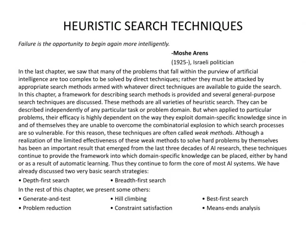
This chapter explores various heuristic search techniques in artificial intelligence, including hill climbing, simulated annealing, and local and global heuristic functions. Learn how these methods can be applied in production systems and working memory, with examples and algorithms provided. Understand the concepts of goal-driven and data-driven approaches, as well as the challenges such as local maximum, plateau, and ridge encountered in hill climbing problems. Discover how task-specific knowledge and algorithmic decisions play a crucial role in identifying optimal solutions.

E N D
Chapter 3Heuristic Search Techniques 323-670 Artificial Intelligence ดร.วิภาดา เวทย์ประสิทธิ์ภาควิชาวิทยาการคอมพิวเตอร์ คณะวิทยาศาสตร์ มหาวิทยาลัยสงขลานครินทร์
Production System • Working memory • Production set = Rules Figure 5.3 • Trace Figure 5.4 • Data driven Figure 5.9 • Goal driven Figure 5.10 • Iteration # • Working memory • Conflict sets • Rule fired The End Page 2
And-Or Graph a Data driven Goal driven The End b c d e f g Page 3
Generate-and-test • Generate all possible solutions • DFS + backtracking • Generate randomly • Test function yes/no • Algorithm page 64 The End Page 4
Hill Climbing • Similar to generate-and-test • Test function + heuristic function • Stop • Goal state meet • No alternative state to move The End Page 5
Simple Hill Climbing • Task specific knowledge into the control process • Is one state better than another • The first state is better than the current state • Algorithm page 66 The End Page 6
Steepest-Ascent Hill Climbing • Consider all moves from the current state • Select the best one as the next state • Algorithm page 67 • Searching time? The End Page 7
Hill Climbing Problem • No solution found : Problem • Local maximum : a state that is better than all its neighbors but it is not better than some other states farther away. • backtracking • Plateau : a flat area of the search space in which a whole set of neighboring states have the same value. It is not possible to determine the best direction by using local comparison. • Make big jump The End Page 8
Hill Climbing Problem • Ridge : an area of the search space that is higher than surrounding areas and itself has a slope. We can not do with a single move. • Fired more rules for several direction The End Page 9
Hill Climbing Characteristic • Local method • It decides what to do next by looking only at the immediate consequences of its choice (rather than by exhaustively exploring all of the consequence) • Look only one more ahead The End Page 10
Local heuristic function • Block world figure 3.1 p. 69 • Local heuristic function 1. Add one point for every block that is resting on the thing it is supposed to be resting on. 2. Subtract one point for every block that is sitting on the wrong thing. • Initial state score = 4 (6-2) • C,D,E,F,G,H correct = 6 • A,B wrong = -2 • Goal state score = 8 • A,B,C,D,E,F,F,H all correct The End Page 11
Local heuristic function • Current state: จากรูป 3.1 • หยิบ A วางบนโต๊ะ B C D E F G H วางเรียงเหมือนเดิม • Score = 6 (B C D E F G Hcorrect) • Block world figure 3.2 p. 69 • Next state score = 4 • All 3 cases • Stop : no better score than the current state = 6 • Local minimum problem • ติดอยู่ในกลุ่มระดับ local มองไปไม่พ้นอ่าง The End Page 12
Global heuristic function • Block world figure 3.1 p. 69 • Global heuristic function • For each block that has the correct support structure add one point for every block in the support structure. (นับหมด) • For each block that has an incorrect support structure, subtract one point for every block in the existing support structure. The End Page 13
Global heuristic function • initial state score = -28 • C = -1, D = -2, E = -3, F = -4, G = -5, H = -6, A = -7 • Goal state score = 28 • B = 1, C = 2, D = 3, E = 4, F = 5, G = 6, H = 7 The End Page 14
Global heuristic function • Current state: จากรูป 3.1 • หยิบ A วางบนโต๊ะ B C D E F G H วางเรียงเหมือนเดิม • Score = -21 • (C = -1, D = -2, E= -3, F = -4, G= -5, H = -6) • Block world figure 3.2 p. 69 • Next state : move to case(c) • Case(a) = -28 same as initial state • Case(b) =-16 • (C = -1, D = -2, E= -3, F = -4, G= -5, H = -1) • Case(c) =-15 • (C = -1, D = -2, E= -3, F = -4, G= -5) • No Local minimum problem It’s work The End Page 15
New heuristic function 1. Incorrect structure are bad and should be taken apart. More subtract score 2. Correct structure are good and should built up. • Add more score for the correct structure. • สิ่งที่เราต้องพิจารณา • How to find a perfect heuristic function? • เข้าไปในเมองที่ไม่เคยไปจะหลีกเลี่ยงทางตัน dead end ได้อย่างไร The End Page 16
Simulated Annealing • Hill climbing variation • At the beginning of the process some down hill moves may be made. • Do enough exploration of the whole space early on so that the final solution is relatively insensitive to the starting state. • ป้องกันปัญหา local maximum, plateau,ridge • Use objective function (not heuristic function) • Use minimize value of objective function The End Page 17
Simulated Annealing • Annealing schedule • ถ้าเราทำให้เย็นเร็วมาก จะได้ผลลัพธ์ high energy อาจเกิด local minimum ได้ • ถ้าเราทำให้เย็นช้ามาก จะได้ผลลัพธ์ดี แต่เสียเวลามาก at low temperatures a lot of time may be wasted after the final structure has already been formed. • ควรทำแบบพอดี empirical structure The End Page 18
Simulated Annealing • Annealing : metals are melted • Cool down to get the solid structure • Objective function : energy level • Try to use less energy • P : probability • T : temperature : annealing schedule • K : Boltzmann’s constant : describe the correspondence between the units of temperature and the unit of energy • E = ( value of current) – (value of new state) • positive change in the energy The End - e/KT p = e Page 19
Simulated Annealing The End • Probability of a large uphill move is lower than probability of a small uphill move • Probability uphill move decrease when temperature decrease. • In the beginning of the annealing large upward moves may occur early on • Downhill moves are allowed anytime • Only relative small upward moves are allowed until finally the process converges to a local minimum configuration Page 20
Simulated Annealing The End - e/KT p = e Page 21
Algorithm Simulated Annealing เหมาะสำหรับปัญหาที่มีจำนวน move มากๆหลักการ1. What is initial Temperature2. Criteria for decreasing T3. Level to decrease T value4. When to quitข้อสังเกต1. When T approach 0 simulated annealing identical with simple hill climbing The End Page 22
Algorithm Simulated Annealing ข้อแตกต่างAlgorithm Simulated Annealing p.71 และHill Climbing1. The annealing schedule must be maintained.2. Move to worse states may be accepted.3. Maintain the best state found so far. If the final state is worse than that earlier state, then earlier state is still available. The End Page 23
Best first search • OR GRAPH : Search in the graph The End Heuristic function : min value page 74 Page 24
Best First Search • OR GRAPH : each of its branches represents an alternative problem-solving pattern • we assumed that we could evaluate multiple paths to the same node independently of each other • we want to find a single path to the goal • use DFS : select most promising path • use BSF : when no promising path/ switch part to receive the better value • old branch is not forgotten • solution can be find without all completing branches having to expanded Page 25
Best First Search f’ = g + h’g: cost from initial state to current stateh’: estimate cost current state to goal state f’: estimate cost initial state to goal state Open node: most promising node Close node : keep in memory, already discover node. Page 26
Best First Search Algorithm page 75-76 Page 27
A* algorithm The End • h’ : count the nodes that we step down the path, 1 level down = 1 point, except the root node. • Underestimate : we generate up until f’(F)= 6 > f’(C) =5 then we have to go back to C. f’ = g + h’ 1 level f’(E) = f’(C) = 5 2 level 3 level Page 28
A* algorithm Overestimate : Suppose the solution is under D : we will not generate D because F’(D) = 6 > f’(G) = 4. The End f’ = g + h’ 1 level 2 level 3 level Page 29
A* Algorithm page 76 Page 30
A* Algorithm Page 31
Agenda • Agenda : a list of tasks a system could perform. • a list of reasons • a rating representing overall weight of evidence suggesting that the task would be useful • When a new task is created, insert into the agenda in its proper place, we need to re-compute its rating and move it to the correct place in the list • find the better location • put at the end of agenda • need a lot more time to compute a new rating The End Page 32
Not acceptable dialog • agenda is not good for when interacting with people page 81-82 • person...............China......... computer............................. • person...............Italy.......... • computer.............................. • person................................... • computer.........China.......... • something reasonable now may not be continue to be so after the conversation has processed for a while. The End Page 33
Agenda The End Page 34
And-Or Graph / Tree • can be solved by decomposing them into a set of smaller problems • And arcs are indicated with a line connecting all the components The End Page 35
And-Or Graph / Tree • each arc with the successor has a cost of 1 The End 9+27+1+1 3+4+1+1 15+10+1+1 choose lowest value = f’(B) = 5 ABEF = 17 + 1 Page 36
And-Or Graph / Tree • Futility : some value use to compare the result/ threshold value • If... the estimate cost of a solution>Futility then.....abandon the search The End Page 37
Problem Reduction The End Page 38
Problem Reduction The End E come from J not C Page 39
Problem Reduction The End Can not find a solution from this algorithm because of C Page 40
Problem Reduction : AO* Algorithm The End Page 41
Problem Reduction : AO* Algorithm • use a single structure GRAPH • we will not store g • algorithm will insert all ancestor nodes into a set path C will always be better than path B Page 42
Problem Reduction : AO* Algorithm change G from 5 to 10 no backward propagation need backward propagation Page 43