Download

1 / 45
450 likes | 487 Views
Explore heuristic search methods, depth-first search, problem reduction, and more to efficiently solve complex problems in AI. Understand how human problem-solving processes are converted into computational steps. Discover the principles and strategies behind heuristic evaluation functions.

E N D
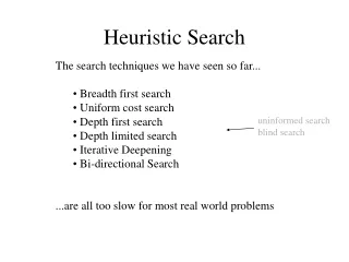
Heuristics • To solve larger problems, domain-specific knowledge must be provided to improve the search efficiency • Heuristic • Any advice that is often effective but is not always guaranteed to work • Heuristic Evaluation Function • Estimates cost of an optimal path between two states • Must be inexpensive to calculate • h(n)
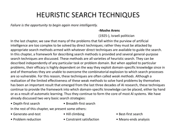
Heuristic Search techniques • There are a number of methods used in Heuristic Search techniques • Depth Search • Breadth Search • Hill climbing • Generate-and-test • Best-first-search • Problem reduction • Constraint satisfaction • Means-ends analysis
Searching and AI • Searching falls under Artificial Intelligence (AI). • A major goal of AI is to give computers the ability to think, or in other words, mimic human behavior. • The problem is, unfortunately, computers don't function in the same way our minds do. • They require a series of well-reasoned out steps before finding a solution.
Searching and AI • Your goal, then, is to take a complicated task and convert it into simpler steps that your computer can handle. • That conversion from something complex to something simple which computer can easily solve.
Searching and AI • Let's first learn how we humans would solve a search problem. • First, we need a representation of how our search problem will exist. • We normally use search tree for representation of how search problem will exist. • It is a series of interconnected nodes that we will be searching through • Let us see diagram below
Searching and AI • In our above graph, the path connections are not two-way. All paths go only from top to bottom. In other words, A has a path to B and C, but B and C do not have a path to A.
Searching and AI • Each lettered circle in our graph is a node. • A node can be connected to other via our edge/path, and those nodes that its connects to are called neighbors. • B and C are neighbors of A. E and D are neighbors of B, and B is not a neighbors of D or E because B cannot be reached using either D or E. • Our search graph also contains depth:
Searching and AI • We now have a way of describing location in our graph. • We know how the various nodes (the lettered circles) are related to each other (neighbors), and we have a way of characterizing the depth each belongs in.
Depth First Search • Depth first search works by taking a node, checking its neighbors, expanding the first node it finds among the neighbors, checking if that expanded node is our destination, and if not, continue exploring more nodes. • Consider the following demonstration of finding a path between A and F:
Depth First Search • Step 0Let's start with our root/goal node: • We can use two lists to keep track of what we are doing - an Open list and a Closed List. An Open list keeps track of what you need to do, and the Closed List keeps track of what you have already done. Right now, we only have our starting point, node A. We haven't done anything to it yet, so let's add it to our Open list.
Depth First Search • Open List: A • Closed List: <empty> • Step 1Now, let's explore the neighbors of our A node. To put another way, let's take the first item from our Open list and explore its neighbors:
Depth First Search • Node A's neighbors are the B and C nodes. Because we are now done with our A node, we can remove it from our Open list and add it to our Closed List. You aren't done with this step though. You now have two new nodes B and C that need exploring. Add those two nodes to our Open list
Depth First Search • Our current Open and Closed Lists contain the following data: • Open List: B, C • Closed List: A • Step 2Our Open list contains two items. For depth first search and breadth first search, you always explore the first item from our Open list. The first item in our Open list is the B node. B is not our destination, so let's explore its neighbors:
Depth First Search • Because we have now expanded B, we are going to remove it from the Open list and add it to the Closed List. Our new nodes are D and E, and we add these nodes to the beginning of our Open list: • Open List: D, E, C • Closed List: A, B
Depth First Search • Because D is at the beginning of our Open List, we expand it. D isn't our destination, and it does not contain any neighbors. All you do in this step is remove D from our Open List and add it to our Closed List: • Open List: E, C • Closed List: A, B, D
Depth First Search • Step 4We now expand the E node from our Open list. E is not our destination, so we explore its neighbors and find out that it contains the neighbors F and G. Remember, F is our target, but we don't stop here though. Despite F being on our path, we only end when we are about to expand our target Node - F in this case
Depth First Search • Our Open list will have the E node removed and the F and G nodes added. The removed E node will be added to our Closed List: • Open List: F, G, C • Closed List: A, B, D, E
Depth First Search • Step 5We now expand the F node. Since it is our intended destination, we stop:
Depth First Search • We remove F from our Open list and add it to our Closed List. Since we are at our destination, there is no need to expand F in order to find its neighbors. • Our final Open and Closed Lists contain the following data: • Open List: G, C • Closed List: A, B, D, E, F
Depth First Search • The final path taken by our depth first search method is what the final value of our Closed List is: A, B, D, E, F.
Breadth First Search • Depth and breadth first search methods are both similar. In depth first search, newly explored nodes were added to the beginning of your Open list. In breadth first search, newly explored nodes are added to the end of your Open list.
Breadth First Search • Let's see how that change will affect our results. Consider the search tree below • Find a path between nodes A and E.
Breadth First Search • Step 0Let's start with our root/goal node: • We will continue to employ the Open and Closed Lists to keep track of what needs to be done: • Open List: A • Closed List: <empty>
Breadth First Search • Step 1Let's explore the neighbors of our A node. So far, we are following in depth first's foot steps: • Remove A from Open list and add A to Closed List. A's neighbors, the B and C nodes, are added to our Open list. They are added to the end of our Open list, but since our Open list was empty (after removing A), it's hard to show that in this step.
Breadth First Search • Current Open and Closed Lists contain the following data: • Open List: B, C • Closed List: A • Step 2Things start to diverge from depth first search method in this step. We take a look the B node because it appears first in our Open List.
Breadth First Search • Because B isn't intended destination, we explore its neighbors: • B is now moved to Closed List, but the neighbors of B, nodes D and E are added to the end of Open list: • Open List: C, D, E • Closed List: A, B
Breadth First Search • Step 3We expand C node: • Since C has no neighbors, all we do is remove C from our Closed List and move on: • Open List: D, E • Closed List: A, B, C
Breadth First Search • Step 4Similar to Step 3, we expand node D. Since it isn't the destination, and it too does not have any neighbors, we simply remove D from Open list, add D to Closed List, and continue on: • Open List: E • Closed List: A, B, C, D
Breadth First Search • Step 5Because our Open list only has one item, we have no choice but to take a look at node E. Since node E is the destination, we can stop here:
Breadth First Search • Our final versions of the Open and Closed Lists contain the following data: • Open List: <empty> • Closed List: A, B, C, D, E
Generate and Test • The generate-and-test strategy is the simplest of all the approaches. • It consists of the following steps: • Generate a possible solution. For some problems, this means generating a particular point in the problem space. For others, it mens generating a path from a start state. • Test to see if this is actually a solution by comparing the chosen point or the end point of the chosen path to the set of acceptable goal state.
Generate and Test • If solution has been found quit. Otherwise return to step 1. • This procedure could lead to an eventual solution within a short period of time if done systematically. • However if the problem space is very large, the eventual solution may be a very long time.
Generate and Test • The generate-and-test algorithm is a depth-first search procedure since complete solutions must be generated before they can be tested. • It can also operate by generating solutions randomly, but then there is no guarantee that a solution will be ever found. • It is known as the British Museum algorithm in reference to a method of finding object in the British Museum by wandering around.
Generate and Test • For a simple problems, exhaustive generate-and-test is often a reasonable technique. • For problems much harder than this, even heuristic generate-and-test, is not very effective technique. • It is better to be combined with other techniques to restrict the space in which to search even further, the technique can be very effective
Hill Climbing • In hill climbing the basic idea is to always head towards a state which is better than the current one. • So, if you are at town A and you can get to town B and town C (and your target is town D) then you should make a move IF town B or C appear nearer to town D than town A does.
Hill Climbing • The hill-climbing algorithm chooses as its next step the node that appears to place it closest to the goal (that is, farthest away from the current position). • It derives its name from the analogy of a hiker being lost in the dark, halfway up a mountain. Assuming that the hiker’s camp is at the top of the mountain, even in the dark the hiker knows that each step that goes up is a step in the right direction.
Hill Climbing • The simplest way to implement hill climbing is as follows: • Evaluate the initial state. If it is also a goal state, then return it and quit. Otherwise continue with the initial state as the current state. • Loop until a solution is found or until there are no new operators left to be applied in the current state. • Select an operator that has not yet been applied to the current state and apply it to produce new state. • Evaluate the new state
Steepest Hill Climbing • Consider all the moves from the current state and select the best one as te next state. • In steepest ascent hill climbing you will always make your next state the best successor of your current state, and will only make a move if that successor is better than your current state.