HEURISTIC SEARCH
720 likes | 1.01k Views
HEURISTIC SEARCH. Heuristic 1. From Greek heuriskein , “to find” . Of or relating to a usually speculative formulation serving as a guide in the investigation or solution of a problem.

HEURISTIC SEARCH
E N D
Presentation Transcript
Heuristic • 1. From Greek heuriskein, “to find”. • Of or relating to a usually speculative formulation serving as a guide in the investigation or solution of a problem. • Computer Science: Relating to or using a problem-solving technique in which the most appropriate solution of several found by alternative methods is selected at successive stages of a program for use in the next step of the program. • the study of methods and rules of discovery and invention. • 5. In state space search, heuristics are formalized as rules for choosing those branches in a state space that are most likely to lead to an acceptable problem solution.
INTRODUCTION Al problem solvers employ heuristics in two situations:- A problem may not have an exact solution, because of inherent ambiguities in the problem statement or available data. Medical diagnosis is an example of this. A given set of symptoms may have several possible causes. Doctors use heuristics to chose the most likely diagnosis and formulate a plan of treatment.
INTRODUCTION Al problem solvers employ heuristics in two situations:- A problem may not have an exact solution, because of inherent ambiguities in the problem statement or available data. Vision is another example of an inherently inexact problem. Visual scenes are often ambiguous, allowing multiple interpretations of the connectedness, extent and orientation of objects. Optical illusions exemplify these ambiguities. Vision systems use heuristics to select the most likely of several possible interpretations of a given scene.
INTRODUCTION Al problem solvers employ heuristics in two situations:- A problem may have an exact solution, but the computational cost of finding it may be prohibitive. In many problems, state space growth is combinatorially explosive, with the number of possible states increasing exponentially or factorially with the depth of the search. Heuristics handle above problem by guiding the search along the most “promising” path through the space. By eliminating unpromising states and their descendants from consideration, a heuristic algorithm can defeat this combinatorial explosion and find an acceptable solution.
INTRODUCTION Heuristics and the design of algorithms to implement heuristic search have been an important part of artificial intelligence research. Game playing and theorem proving require heuristics to reduce search space to simplify the solution finding. It is not feasible to examine every inference that can be made in search space of reasoning or every possible move in a board game to reach to a solution. In this case, heuristic search provides a practical answer.
INTRODUCTION • Heuristics are fallible. • A heuristics is only an informed guess of the next step to be taken in solving a problem. It is often based on experience or intuition. • Heuristics use limited information, such as the descriptions of the states currently on the open list, they are seldom able to predict the exact behavior of the state space farther along in the search. • A heuristics can lead a search algorithm to a sub optimal solution or fail to find any solution at all.
Tic-Tac-Toe • The combinatorics for exhaustive search are high. • Each of the nine first moves has eight possible responses. • which in turn have seven continuing moves, and so on. • As simple analysis puts exhaustive search at 9 x 8 x7x … or 9!. • Symmetry reduction can decrease the search space, there are really only three initial moves. • To a corner. • To the center of a side. • To the center of the grid.
Tic-Tac-Toe Symmetry reductions on the second level of states further reduce the number of possible paths through the space. In following figure the search space is smaller then the original space but It is still factorial in its growth.
Tic-Tac-Toe • Heuristics • Algorithm analysis the moves in which X has the most winning lines. • Algorithm then selects and moves to the state with the highestheuristic value i.e. X takes the center of the grid.
Figure 4.2:The “most wins” heuristic applied to the first children in tic-tac-toe.
Tic-Tac-Toe • Heuristics • Other alternatives and their descendants are eliminated. • Approximately two-thirds of the space is pruned away with the first move . • After the first move, the opponent can choose either of two alternative moves.
Tic-Tac-Toe • Heuristics • After the move of opponent, The “max win lines” heuristics can be applied to the resulting state of the game. • As search continues, each move evaluates the children of a single node: exhaustive search is not required. • Figure shows the reduced search after three steps in the games. States are marked with their heuristics values.
Tic-Tac-Toe • COMPLAXITY • It is difficult to compute the exact number of states that must be examined. However, a crude upper bound can be computed by assuming a maximum of nine moves in a game and eight children per move. • In reality: • The number of states will be smaller, as board fills and reduces our options. • In addition opponent is responsible for half the moves. • Even this crude upper bound of 8 x 9 or 72 states is an improvement of four orders of magnitude over 9!.
ALGORITHM FOR HEURISTICS SEARCH Implementing Best-First-Search • Best first search uses lists to maintain states: • OPEN to keep track of the current fringe of the search. • CLOSED to record states already visited. • Algorithm orders the states on OPENaccording to some heuristics estimate of their “closeness” to a goal. • Each iteration of the loop consider the most “promising” state on the OPENlist. • Example algorithm sorts and rearrange OPEN in precedence of lowest heuristics value.
BEST-FIRST-SEARCH Figure: Heuristic search of a hypothetical state space with OPEN and CLOSED states highlighted.
BEST-FIRST-SEARCH • At each iteration best-first –search removes the first element from the OPENlist. If it meets the goals conditions, the algorithm returns the solution path that led to the goal. • Each state retains ancestor information to determine if it had previously been reached by a shorter path and to allow the algorithm to return the final solution path. • If the first element on OPEN is not a goal, the algorithm generate its descendants. • If a child state is already on OPEN or CLOSED, the algorithm checks to make sure that the state records the shorter of the two partial solution paths. • Duplicate states are not retained. • By updating the ancestor history of nodes on OPEN and CLOSED when they are rediscovered, the algorithm is more likely to find a shorter path to a goal.
BEST-FIRST-SEARCH • Best-first-search applies a heuristics evaluation to the states on OPEN, and the list is sorted accordingly to the heuristic values of those states. This brings the beststates to the front of OPEN. • Because these estimates are heuristic in nature, the next state to be examined may be from any level of the state space. When OPENis maintained as a sorted list, it is often referred a priority queue. • Figure 4.4 shows a hypothetical state space with heuristic evaluations attached to some of its states. • The goals of best –first search is to find the goals state by looking at as few states as possible: the more informed the heuristic, the fewer states are processed in finding the goal.
BEST-FIRST-SEARCH • The best-first search algorithm always selects the most promising state on OPENfor further expansion. • It does not abandon all the other states but maintains them on OPEN. • In the event a heuristic leads the search down a path that proves incorrect, the algorithm will eventually retrieve some previously generated next best state from OPENand shift its focus to another part of the space. • In the example after the children of state B were found to have poor heuristic evaluations, the search shifted its focus to state C. • In best-first-search the OPENlist allows backtracking from paths that fail to produce a goal.
IMPLEMENTING HEURISTIC EVALUATION FUNCTIONS • We will evaluate performance of various heuristics for solving the 8-puzzle. • Figure shows a start and goal state for the 8-puzzle, along with the first three states generated in the search.
IMPLEMENTING HEURISTIC EVALUATION FUNCTIONS • Heuristic 1 • The simplest heuristic, counts the tiles out of place in each state when it is compared with the goal. • The state that had fewest tiles out of place is probably closer to the desired goal and would be the best to examine next. • However, this heuristic does not use all of the information available in a board configuration, because it does not take into account the distance the tiles must be moved.
IMPLEMENTING HEURISTIC EVALUATION FUNCTIONS • Heuristic 2 • A “better” heuristic would sum all the distances by which the tiles are out of place, one for each square a tile must be moved to reach its position in the goal state.
IMPLEMENTING HEURISTIC EVALUATION FUNCTIONS • Heuristic 3 • Above two heuristics fail to take into account the problem of tile reversals. • If two tiles are next to each other and the goal requires their being in opposite locations, it takes more than two moves to put them back to place, as the tiles must “go around” each other. • A heuristic that takes this into account multiplies a small number (2 , for example) times each direct title reversal.
IMPLEMENTING HEURISTIC EVALUATION FUNCTIONS • The “sum of distances” heuristic provides a more accurate estimate of the work to be done than the “number of titles out of place” heuristic. • Title reversal heuristic gives out an evaluation of ‘0’ since non of these states have any direct tile reversals.
IMPLEMENTING HEURISTIC EVALUATION FUNCTIONS • Devising A Good Heuristic • Good heuristics are difficult to devise. Judgment and intuition help, but the final measure of a heuristic must be its actual performance on problem instances. • Each heuristic proposed above ignores some critical information and needs improvement. • An improved version is discussed next.
IMPLEMENTING HEURISTIC EVALUATION FUNCTIONS • Devising A Good Heuristic • The distance from the starting state to its descendants can be measured by maintaining a depth count for each state. This count is ‘0’ for the beginning state and may be incremented by ‘1’ for each level of the search. • It records the actual number of moves that have been used to go from the starting state in the search to each descendant.
IMPLEMENTING HEURISTIC EVALUATION FUNCTIONS • Devising A Good Heuristic • Let evaluation function ‘f(n)’, be the sum of two components: f(n) = g(n) + h(n) • Where:- • g(n) measures the actual length of the path from start state to any state n. • h(n) is a heuristic estimate of the distance from the state n to a goal.
IMPLEMENTING HEURISTIC EVALUATION FUNCTIONS h(n) = 5 h(n) = 3 h(n) = 5
BEST-FIRST SEARCH GRAPH • Each state is labeled with a letter and its heuristic weight, f(n) = g(n) + h(n). • The number at the top of each state indicates the order in which it was taken off the OPEN list.
Successive stages of OPEN and CLOSED that generates the graph are:
The g(n) component of the evaluation function gives the search more of a breadth-first flavor. • This prevent it from being misled by an erroneous evaluation, If a heuristic continuously returns “good” evaluations for states along a path that fails to reach a goal, the g value will grow to dominate h and force search back to a shorter solution path. • This guarantees that the algorithm will not become permanently lost, descending an infinite branch.
HEURISTIC SEARCH AND EXPERT SYSTEMS • Simple games such as the 8-puzzle are ideal vehicles for exploring the design and behavior of heuristic search algorithms. • More realistic problems greatly complicate the implementation and analysis of heuristic search by requiring multiple heuristics to deal with different situations in the problems space. • A single heuristic may not apply to each state in these domains. • Instead, situation specific problem-solving heuristics are encoded to deal with various states. • Each solution step incorporates its own heuristic that determines when, it should be applied.
EXAMPLE: THE FINANCIAL ADVISOR • An individual with adequate savings and income should invest in stocks. saving_account(adequate)income(adequate)investment(stocks). • The individual may prefer the added security of a combination strategy. saving_account(adequate)income(adequate)investment(combination). • The individual may prefer placing all investment money in savings. saving_account(adequate)income(adequate)investment(savings). • Thus the rule is a heuristic in nature. The problem solver should be programmed to account for this uncertainty. Additional factors may also be taken into account to make the rule more informed and capable of finer distinctions. • Age of the investor. • Long term prospects for security. • Advancement in investors profession.
EXAMPLE: AN EXPERT SYSTEMTHE FINANCIAL ADVISOR • Now how the financial advisor is going to weigh the above heuristic to decide the best option or to find out a solution which is closer to the best solution. • One way is to attach a confidence measure with the conclusion of each rule. Attach a real number between –1 to 1 as:- • 1 corresponding to certainty ‘True’. • -1 to define a value of ‘False’. • Values in between reflect varying confidence levels. • This way the preceding rules would be reflected as under: saving_account(adequate)income(adequate)investment(stocks). with confidence = 0.8 saving_account(adequate)income(adequate)investment(combination). with confidence = 0.5 saving_account(adequate)income(adequate)investment(savings). with confidence = 0.1
ADMISSIBILITY MEASURES • A search algorithm is admissible if it is guaranteed to find a minimal path to solution, whenever such a path exists. • Breadth-first search is an admissible search strategy . • In determining the properties of admissible heuristics, we define an evaluation function f*. f*(n) = g*(n) + h*(n) • Let: f(n) = g(n) + h(n) • g(n) measures the depth(cost) at which state n has been found in the graph. • h(n) is the heuristic estimate of the cost from n to a goal. • f(n) is the estimate of total cost of the path from the start state through node n to the goal state. • Let: f*(n) = g*(n) + h*(n) • g*(n) is the cost of the shortest path from the start node to node n • h*(n) returns the actual cost of the shortest path from n to the goal. • f*(n) is the actual cost of the optimal path from a start node through node n to a goal node.
ADMISSIBILITY MEASURES • In an algorithm A, Ideally function f should be a close estimate of f*. • The cost of the current path, g(n) to state n, is a reasonable estimate of g*(n). • Where: g(n) g*(n). • These are equal only if the graph search has discovered the optimal path to state n. • Similarly, we compare h*(n) with h(n). • h(n) is bounded from above by h*(n) i.e, h(n) is always less than or equal to the actual cost of a minimal path h*(n) i.e. h(n) h*(n). • If algorithm A uses an evaluation function f in which h(n) h*(n), the algorithm is called algorithm A*.
The heuristic of counting the number of tiles out of place is certainly less than or equal to the number of moves required to move them to their goal position. Thus this heuristic is admissible and guarantees an optimal solution path. h(n) h*(n)
Comparison of search using heuristics with search by breadth-first search. • Heuristic used is f(n) = g(n) + h(n) where h(n) is tiles out of place. • The portion of the graph searched heuristically is shaded. The optimal solution path is in bold.
ni nj ng
Monotonic heuristic is admissible. Consider any path in the space as a sequence of states S1, S2, …… Sg, where S1 is the start state and Sg is the goal: For the sequence of moves in this arbitrary selected path: • S1 to S2 h(S1) - h(S2) cost (S1, S2) by monotone property • S2 to S3 h(S2) - h(S3) cost (S2, S3) by monotone property • S3 to S4 h(S3) - h(S4) cost (S3, S4) by monotone property • . . . . by monotone property • . . . . by monotone property • Sg-1 to Sg h(Sg-1) - h(Sg) - cost (Sg-1, Sg) by monotone property • Summing each column and using the monotone property of h(Sg) = 0: • path S1 to Sg h(S1) cost (S1, Sg) • This means that monotone heuristic h is A* and admissible.
If breadth first search is considered a A* algorithm with heuristic h1, then it must be less than h* (as breadth first search is admissible). • Also number of tiles out of place with respect to goal state is a heuristic h2. As this is also admissible therefore, h2 is less than h*. • In this case h1 h2 h*. It follows that the “number of tiles out of place” heuristic is more informed than breadth-first search. • Both h1 and h2 find the optional path, but h2 evaluates many fewer states in the process.
Similarly the heuristic that calculates the sum of the direct distances by which all the tiles are out of place is again more informed than the calculation of the number of tiles are out of place with respect to the goal state. • One can visualize a sequence of search spaces, each smaller than the previous one, converging on the direct optimal path solution. • If a heuristic h2 is more informed then h1 then the set of states examined by h2 is a subset of those examined by h1. • In general, then the more informed and A* algorithm, the less of the space it needs to expand to get the optimal solution.
Figure 4.17:Two-ply minimax applied to the opening move of tic-tac-toe, from Nilsson (1971).
Figure 4.18:Two-ply minimax and one of two possible MAX second moves, from Nilsson (1971).
Figure 4.19:Two-ply minimax applied to X’s move near the end of the game, from Nilsson (1971).
Figure 4.20:Alpha-beta pruning applied to state space of Figure 4.15. States without numbers are not evaluated.