Download
1 / 34
340 likes | 516 Views
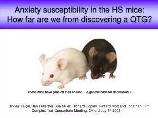
Anxiety susceptibility in the HS mice: How far are we from discovering a QTG?. These mice have gone off their cheese… A genetic basis for depression ?. Binnaz Yal ç ι n, Jan Fullerton, Sue Miller, Richard Copley, Richard Mott and Jonathan Flint

E N D
Anxiety susceptibility in the HS mice: How far are we from discovering a QTG? These mice have gone off their cheese… A genetic basis for depression ? Binnaz Yalçιn, Jan Fullerton, Sue Miller, Richard Copley, Richard Mott and Jonathan Flint Complex Trait Consortium Meeting, Oxford July 1st 2003
95 % CI 0.8 cM Fine-resolution mapping on mouse chromosome 1
143.0 144.0 145.0 146.0 147.0 148.0 D1Mit423 D1Mit499 D1Mit198 D1Mit194 D1Mit100 D1Mit395 D1Mit101 D1Mit264 D1Mit102 Markers 0.8 cM FISH cM 73.0 73.1 73.2 73.4 73.5 73.7 74.0 73.3 73.8 73.9 cR 15.0 16.0 17.0 18.0 Mb Mouse chromosome 1
Rgs1p21ex5 16.84FRF7 212I24T 278P12T 132C16T 278M14S 278M14T 101B24S 231L2S 231L2T 329H3T 4K20T 90A8S 37J4S 37J4T 311I21 436B15 146B4 368O20 278M14 212I24 305E1 480H2 134A16 282N6 445F7 129N3 90A8 285F13 238L2 206E19 132C16 174G1 185E17 220K2 447B15 7I3 4K20 101B24 431N20 37J4 329H3 231L2 459A11 278P12 D1Mit423 D1Mit499 D1Mit198 D1Mit194 238K21 D1Mit100 D1Mit395 D1Mit101 D1Mit264 D1Mit102 Markers 0.8 cM FISH cM 73.0 73.1 73.2 73.4 73.5 73.7 74.0 73.3 73.8 73.9 cR 15.0 16.0 17.0 18.0 Mb 143.0 144.0 145.0 146.0 147.0 148.0 Mouse chromosome 1 A 4.8-Mb high-resolution integrated BAC-based map MMHAP94
Approaches used to identify genes 1. Find expressed sequence tags (ESTs) using BLAST alignment 2. Compare with other species
How many genes would you expect in a 4.8-Mb region?
Glrx2 RGS2 B302775 SSA2 RGS13 B3Galt2 RGS18 B830045N13 UCHL5 RGS1 • B3Galt2 (Beta 1,3-Galactosyltransferase 2). • Glrx2 (Glutaredoxin 2) also known as thioltransferase. • SSA2 (Sjögren Syndrome Autoantigen). • UCHL5 (Ubiquitin C-Terminal Hydrolase L5). • 2 unknown ESTs (B302775 and B830045N13), respectively CDC73 and retinoic acid inducible neural specific protein homologues. • 4 RGS genes (Regulator of G protein Signalling). Only 10 expressed sequences found Mb 143.0 144.0 145.0 146.0 147.0 148.0
Have we missed any expressed sequences ?
The Fugu genome is ideal for gene discovery in vertebrates • It contains a similar number of genes with short intergenic regions. • It spans 365-Mb which has been sequenced to over 95 % coverage.
Mouse-Fugu comparison • 4.8 Mb were aligned to the whole Fugu genome. • Significant hits were identified. • Are there any new matches that are explained by unidentified expressed sequences? • All the hits found correspond to the genes previously identified. • We haven't missed any coding sequence.
Are there any variants in these genes?
Identification of variants • We sequenced all the genes we previously identified in each of the HS founder strains and also in 12 HS mice. • We covered coding sequences for all the genes. • All RGS genes were fully sequenced including 4 Kb in the 5’ UTR and 2Kb in the 3’ UTR.
Sequencing results for RGS2 RGS1 and RGS18 RGS2 Polymorphisms 7145 bp Structure 1 2 3 4 5 22 polymorphisms Coverage 100 % coverage Scale 0 2.0 4.0 6.0 8.0 Polymorphisms RGS1 Structure 1 2 3 4 5 7368 bp Coverage 96 polymorphisms Scale 100 % coverage 0 1.0 2.0 3.0 4.0 5.0 6.0 7.0 8.0 9.0 10.0 RGS18 Polymorphisms Structure 22592 bp 1 2 3 4 5 Coverage 49 polymorphims 100 % coverage Scale 0 2.5 5.0 7.5 10.0 12.5 15.0 17.5 20.0 22.5 25.0 Coding variants SNP Exons del/ins repeats Coverage
Summary of gene sequencing • We sequenced 100 Kb in each of the 8 HS founders and in 12 HS mice. • We found 296 polymorphisms. • 81% were SNPs, 13 % repeats and 6% ins/del. • Average polymorphism rate is 1 per 200 bp. • We observed segments of high (1 per 50 bp) and low (1 per 500 bp) polymorphism rates. • All the polymorphisms found in the HS founders are also present in the HS mice.
Summary • 0.8 cM contains 4.8 Mb DNA. • 10 genes were identified in 4.8 Mb. • 3 genes have coding variants, none of which are predicted to alter the gene’s function. • We cannot find any mutations that disrupt gene function.
How can we identify functionally important non-coding variants?
Sequencing conserved non-coding regions • We found over 600 conserved non-coding regions using 70% identity over 100 bp regions. • We sequenced 20% of the conserved non-coding regions, representing 120 Kb of sequencing in each of the HS founder strains. • Extrapolating, we predicted that there are over 1000 polymorphisms in the 4.8 Mb region.
What is the arrangement of polymorphisms across the genomes of the 8 HS founders ?
Polymorphisms found in the HS founders • Primers spaced on average every 5-10 Kb. • All polymorphisms detected by sequencing. • 1219 polymorphisms found including 76 % SNPs, 14% del/ins and 10 % repeat polymorphisms. • Average polymorphism density is 1 per 5 Kb.
AJ/C57 Number of variants/100 Kb Physical distance BALB/C57 Number of variants/100 Kb Physical distance I/RIII Number of variants/100 Kb Physical distance Examples of pairwise comparison of inbred strains
Summary of variants found • 8 in coding regions. • 80 in 5’ UTR. • 208 in introns. • 1000 in conserved non-coding regions. • 713 in non-conserved regions.
What is the probability that a variant influences the phenotype ?
Assigning probabilities to variants • We originally identified QTL by testing for differences between the 8 HS founder strains, allowing each strain to have a different trait value. • But a SNP merges the founder strains into two groups. • If the SNP is the QTN then forcing those strains within a group to have the same trait value in the statistical test will be as good. • If the test is non-significant then we can exclude that SNP as candidate.
Physical distance (Mb) HAPPY results across our whole region
RGS2 RGS13 RGS18 RGS1 Glrx2 SSA2 B3 B3Galt2 B8 UCHL5 Physical distance (Mb) HAPPY results across our whole region
Most significant SNPs lie within a conserved non-coding region
How many variants could we exclude? • We can exclude 77% of the SNPs identified that are not significant. • Among coding variants none is significant. • Among 5’ UTR regions 17 are significant. • We can further exclude another 13 % which lie under non-conserved regions. • This identifies 120 SNPs as significant.
Conclusions • There are no obvious coding variants that are the QTN. • Haplotype analysis can help limit the search but involves immense amounts of sequencing. • There may not be a single responsible variant. • One region, 5’ of the RGS18 gene contains the most significant SNPs, within a conserved non-coding region
Jonathan Flint • Richard Mott • Jan Fullerton • Sue Miller • Andrew Morris • Richard Copley • John Broxholme Acknowledgements