Lecture 13 - Heat Transfer Applied Computational Fluid Dynamics
390 likes | 1.09k Views
Lecture 13 - Heat Transfer Applied Computational Fluid Dynamics. Instructor: André Bakker. © André Bakker (2002-2004) © Fluent Inc. (2002). Introduction. Typical design problems involve the determination of: Overall heat transfer coefficient, e.g. for a car radiator.

Lecture 13 - Heat Transfer Applied Computational Fluid Dynamics
E N D
Presentation Transcript
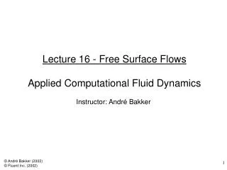
Lecture 13 - Heat TransferApplied Computational Fluid Dynamics Instructor: André Bakker © André Bakker (2002-2004) © Fluent Inc. (2002)
Introduction • Typical design problems involve the determination of: • Overall heat transfer coefficient, e.g. for a car radiator. • Highest (or lowest) temperature in a system, e.g. in a gas turbine, chemical reaction vessels, food ovens. • Temperature distribution (related to thermal stress), e.g. in the walls of a spacecraft. • Temperature response in time dependent heating/cooling problems, e.g. engine cooling, or how fast does a car heat up in the sun and how is it affected by the shape of the windshield?
Modes of heat transfer • Conduction: diffusion of heat due to temperature gradients. A measure of the amount of conduction for a given gradient is the heat conductivity. • Convection: when heat is carried away by moving fluid. The flow can either be caused by external influences, forced convection; or by buoyancy forces, natural convection. Convective heat transfer is tightly coupled to the fluid flow solution. • Radiation: transfer of energy by electromagnetic waves between surfaces with different temperatures, separated by a medium that is at least partially transparent to the (infrared) radiation. Radiation is especially important at high temperatures, e.g. during combustion processes, but can also have a measurable effect at room temperatures.
Overview dimensionless numbers • Nusselt number: Ratio between total heat transfer in a convection dominated system and the estimated conductive heat transfer. • Grashof number: Ratio between buoyancy forces and viscous forces. • Prandtl number: Ratio between momentum diffusivity and thermal diffusivity. Typical values are Pr = 0.01 for liquid metals; Pr = 0.7 for most gases; Pr = 6 for water at room temperature. • Rayleigh number: The Rayleigh number governs natural convection phenomena. • Reynolds number: Ratio between inertial and viscous forces.
Enthalpy equation • In CFD it is common to solve the enthalpy equation, subject to a wide range of thermal boundary conditions. • Energy sources due to chemical reaction are included for reacting flows. • Energy sources due to species diffusion are included for multiple species flows. • The energy source due to viscous heating describes thermal energy created by viscous shear in the flow.This is important when the shear stress in the fluid is large (e.g. lubrication) and/or in high-velocity, compressible flows. Often, however, it is negligible. • In solid regions, a simple conduction equation is usually solved, although convective terms can also be included for moving solids.
“Conjugate heat transfer” refers to the ability to compute conduction of heat through solids, coupled with convective heat transfer in a fluid. Coupled boundary conditions are available for wall zones that separate two cell zones. Either the solid zone or the fluid zone, or both, may contain heat sources. The example here shows the temperature profile for coolant flowing over fuel rods that generate heat. Grid Velocity vectors Temperature contours Example: Cooling flow over fuel rods Conjugate heat transfer
The heat flux is proportional to the temperature gradient: where k(x,y,z,T) is the thermal conductivity. In most practical situations conduction, convection, and radiation appear in combination. Also for convection, the heat transfer coefficient is important, because a flow can only carry heat away from a wall when that wall is conducting. temperature profile hot wall cold wall x Heat conduction - Fourier’s law
heat conduction in heat conduction out T heat generation rate of change of temperature heat cond. in/out heat generation thermal diffusivity Generalized heat diffusion equation • If we perform a heat balance on a small volume of material…. • … we get:
Tout = 20°F Tout = 68°F Although slight, you can see the “thermal bridging” effect through the studs 2x6 stud k=0.15 W/m2-K sheetrock k=0.4 W/m2-K shingles k=0.15 W/m2-K fiberglass insulation k=0.004 W/m2-K sheathing k=0.15 W/m2-K Conduction example • Compute the heat transfer through the wall of a home:
flow over a heated block Convection heat transfer • Convection is movement of heat with a fluid. • E.g., when cold air sweeps past a warm body, it draws away warm air near the body and replaces it with cold air.
Forced convection example • Developing flow in a pipe (constant wall temperature). T bulk fluid temperature heat flux from wall x
thermal boundary layer edge velocity boundary layer edge y Thermal boundary layer • Just as there is a viscous boundary layer in the velocity distribution, there is also a thermal boundary layer. • Thermal boundary layer thickness is different from the thickness of the (momentum) viscous sublayer, and fluid dependent. The thickness of the thermal sublayer for a high-Prandtl-number fluid (e.g. water) is much less than the momentum sublayer thickness. For fluids of low Prandtl numbers (e.g. liquid metal), it is much larger than the momentum sublayer thickness.
Natural convection (from a heated vertical plate). As the fluid is warmed by the plate, its density decreases and a buoyant force arises which induces flow in the vertical direction. The force is proportional to The dimensionless group that governs natural convection is the Rayleigh number: Typically: T Tw u gravity Natural convection
Light weight warm air tends to move upward when surrounded by cooler air. Thus, warm-blooded animals are surrounded by thermal plumes of rising warm air. This plume is made visible by means of a Schlieren optical system that is based on the fact that the refraction of light through a gas is dependent on the density of the gas. Although the velocity of the rising air is relatively small, the Reynolds number for this flow is on the order of 3000. Natural convection around a person
Natural convection - Boussinesq model • Makes simplifying assumption that density is uniform. • Except for the body force term in the momentum equation, which is replaced by: • Valid when density variations are small (i.e. small variations in T). • Provides faster convergence for many natural-convection flows than by using fluid density as function of temperature because the constant density assumptions reduces non-linearity. • Natural convection problems inside closed domains: • For steady-state solver, Boussinesq model must be used. Constant density o allows mass in volume to be defined. • For unsteady solver, Boussinesq model or ideal gas law can be used. Initial conditions define mass in volume.
q Tbody average heat transfer coefficient (W/m2-K) Newton’s law of cooling • Newton described the cooling of objects with an arbitrary shape in a pragmatic way. He postulated that the heat transfer Q is proportional to the surface area A of the object and a temperature difference T. • The proportionality constant is the heat transfer coefficient h(W/m2-K). This empirical constant lumps together all the information about the heat transfer process that we don’t know or don’t understand.
h is not a constant, but h = h(DT). Three types of convection. Natural convection. Fluid moves due to buoyancy. Forced convection: flow is induced by external means. Boiling convection: body is hot enough to boil liquid. Typical values of h: Thot Tcold 4 - 4,000 W/m2-K Tcold 80 - 75,000 Thot Tcold 300 - 900,000 Thot Heat transfer coefficient
Radiation heat transfer • Thermal radiation is emission of energy as electromagnetic waves. • Intensity depends on body temperature and surface characteristics. • Important mode of heat transfer at high temperatures, e.g. combustion. • Can also be important in natural convection problems. • Radiation properties can be strong functions of chemical composition, especially CO2, H2O. • Radiation heat exchange is difficult solve (except for simple configurations). We must rely on computational methods.
(W/m2) (incident energy flux) (reflected) (absorbed) translucent slab (transmitted) absorptance transmittance reflectance Surface characteristics
Black body radiation • A “black body”: • Is a model of a perfect radiator. • Absorbs all energy that reaches it; reflects nothing. • Therefore • The energy emitted by a black body is the theoretical maximum: • This is Stefan-Boltzmann law; s is the Stefan-Boltzmann constant (5.6697E-8 W/m2K4). • The wavelength at which the maximum amount of radiation occurs is given by Wien’s law: • Typical wavelengths are max = 10 m (far infrared) at room temperature andmax = 0.5 m (green) at 6000K.
Real bodies • Real bodies will emit less radiation than a black body: • Here is the emissivity, which is a number between 0 and 1. Such a body would be called “gray” because the emissivity is the average over the spectrum. • Example: radiation from a small body to its surroundings. • Both the body and its surroundings emit thermal radiation. • The net heat transfer will be from the hotter to the colder. • The net heat transfer is then: • For small T the term (Tw4-T4) can be approximated as and with hr as an effective radiation heat transfer coefficient.
Radiation • Radiation intensity transport equations (RTE) are solved. • Local absorption by fluid and at boundaries links energy equation with RTE. • Radiation intensity is directionally and spatially dependent. • Intensity along any direction can be reduced by: • Local absorption. • Out-scattering (scattering away from the direction). • Intensity along any direction can be augmented by: • Local emission. • In-scattering (scattering into the direction). • Four common radiation models are: • Discrete Ordinates Model (DOM). • Discrete Transfer Radiation Model (DTRM). • P-1 Radiation Model. • Rosseland Model.
Heat transfer optimization • We have the following relations for heat transfer: • Conduction: • Convection: • Radiation: • As a result, when equipment designers want to improve heat transfer rates, they focus on: • Increasing the area A, e.g. by using profiled pipes and ribbed surfaces. • Increasing T (which is not always controllable). • For conduction, increasing kf /d. • Increase h by not relying on natural convection, but introducing forced convection. • Increase hr, by using “black” surfaces.
Fluid properties • Fluid properties such as heat capacity, conductivity, and viscosity can be defined as: • Constant. • Temperature-dependent. • Composition-dependent. • Computed by kinetic theory. • Computed by user-defined functions. • Density can be computed by ideal gas law. • Alternately, density can be treated as: • Constant (with optional Boussinesq modeling). • Temperature-dependent. • Composition-dependent. • User defined functions.
Systems in which phase change occurs (e.g. melting, solidification, and sometimes evaporation) can be modeled as a single-phase flow with modified physical properties. In that case, the medium gets the properties of one phase state below a certain critical temperature, and the properties of the other phase state above a second critical temperature. Linear transitions for and . A “spike” in cp is added, the area of which corresponds to the latent heat. A second spike is added to the heat conductivity curve, to keep the ratio between heat capacity and thermal conductivity constant. latent heat heat capacity density conductivity viscosity Temperature Phase change
Thermal boundary conditions • At flow inlets and exits. • At flow inlets, must supply fluid temperature. • At flow exits, fluid temperature extrapolated from upstream value. • At pressure outlets, where flow reversal may occur, “backflow” temperature is required. • Thermal conditions for fluids and solids. • Can specify energy source. • Thermal boundary conditions at walls. • Specified heat flux. • Specified temperature. • Convective heat transfer. • External radiation. • Combined external radiation and external convective heat transfer.
Notes on convergence • Heat transfer calculations often converge slowly. It is recommended to use underrelaxation factors of 0.9 or larger for enthalpy. If lower underrelaxation factors are used, obtaining a good solution may take prohibitively long. • If underrelaxation factors of 0.2 or lower have to be used to prevent divergence, it usually means that the model is ill-posed. • Deep convergence is usually required with scaled residuals having to be of the order 1E-6 or smaller.
Problem: improve the efficiency of a tube-cooled reactor. Non-standard design, i.e. traditional correlation based methods not applicable. Solution: more uniform flow distribution through the shell that will result in a higher overall heat transfer coefficient and improved efficiency. Example: heat exchanger efficiency
Original design: Bundle of tubes as shown. Repeated geometry. 3 different baffles, A, C, and D. Reactant injectors between baffles “A” and “D”. mm mmmmm mmmmmmm mmmmmmmmmmmmmmmmmmmmmmmmmmmmmmmmmmmmmmmmmmmmmmmmmmmmmmmmmmmmmmmmmmmmmmmmmmmmmmmmmmmmmmmmmmmmmmmmmmmmmmmmmmmmmmmmmmmmmm mmmm m mm mmmmm mmmmmmm mmmmmmmmmmmmmmmmmmmmmmmmmmmmmmmmmmmmmmmmmmmmmmmmmmmmmmmmmmmmmmmmmmmmmmmmmmmmmmmmmmmmmmmmmmmmmmmmmmmmmmmmmmmmmmmmmmmmmm mmmm m mm mmmmm mmmmmmm mmmmmmmmmmmmmmmmmmmmmmmmmmmmmmmmmmmmmmmmmmmmmmmmmmmmmmmmmmmmmmmmmmmmmmmmmmmmmmmmmmmmmmmmmmmmmmmmmmmmmmmmmmmmmmmmmmmmmm mmmm m mm mmmmm mmmmmmm mmmmmmmmmmmmmmmmmmmmmmmmmmmmmmmmmmmmmmmmmmmmmmmmmmmmmmmmmmmmmmmmmmmmmmmmmmmmmmmmmmmmmmmmmmmmmmmmmmmmmmmm mmmm m Flow Direction mm mmmmm mmmmmmm mmmmmmmmmmmmmmmmmmmmmmmmmmmmmmmmmmmmmmmmmmmmmmmmmmmmmmmmmmmmmmmmmmmmmmmmmmmmmmmmmmmmmmmmmmmmmmmmmmmmmmmmmmmmmmmmmmmmmm mmmm m mm mmmmm mmmmmmm mmmmmmmmmmmmmmmmmmmmmmmmmmmmmmmmmmmmmmmmmmmmmmmmmmmmmmmmmmmmmmmmmmmmmmmmmmmmmmmmmmmmmmmmmmmmmmmmmmmmmmmmmmmmmmmmmmmmmm mmmm m Heat exchanger - original design Baffle “A” Injectors Baffle “C” Baffle “D”
3-dimensional, steady, turbulent, incompressible, isothermal. Bundle of tubes modeled as a non-isotropic porous medium. Two symmetry planes significantly reduce domain size. Hybrid, unstructured mesh of 330,000 cells. Zero thickness walls for baffles. Leakage between baffles and shell wall (0.15” gap) modeled using thin prism cells. Uniform inflow applied over a half-cylindrical surface upstream of the first baffle. Heat exchanger - modeling approach
D A C A D A C A D Bundle of tubes (Shaded area) Flow Direction Injection points Compartment mainly served by nearest upstream injector Compartments with low flow Non-uniform flow distribution means low efficiency Heat exchanger - flow pattern Recirculation loops
Design modifications: Shorter baffles “ C’ ”. Relocated and rotated injectors. mm mmmmm mmmmmmm mmmmmmmmmmmmmmmmmmmmmmmmmmmmmmmmmmmmmmmmmmmmmmmmmmmmmmmmmmmmmmmmmmmmmmmmmmmmmmmmmmmmmmmmmmmmmmmmmmmmmmmmmmmmmmmmmmmmmm mmmm m mm mmmmm mmmmmmm mmmmmmmmmmmmmmmmmmmmmmmmmmmmmmmmmmmmmmmmmmmmmmmmmmmmmmmmmmmmmmmmmmmmmmmmmmmmmmmmmmmmmmmmmmmmmmmmmmmmmmmmmmmmmmmmmmmmmm mmmm m Relocated Injectors Modified (Shorter) Baffle “ C’ ” mm mmmmm mmmmmmm mmmmmmmmmmmmmmmmmmmmmmmmmmmmmmmmmmmmmmmmmmmmmmmmmmmmmmmmmmmmmmmmmmmmmmmmmmmmmmmmmmmmmmmmmmmmmmmmmmmmmmmmmmmmmmmmmmmmmm mmmm m mm mmmmm mmmmmmm mmmmmmmmmmmmmmmmmmmmmmmmmmmmmmmmmmmmmmmmmmmmmmmmmmmmmmmmmmmmmmmmmmmmmmmmmmmmmmmmmmmmmmmmmmmmmmmmmmmmmmmm mmmm m Flow Direction mm mmmmm mmmmmmm mmmmmmmmmmmmmmmmmmmmmmmmmmmmmmmmmmmmmmmmmmmmmmmmmmmmmmmmmmmmmmmmmmmmmmmmmmmmmmmmmmmmmmmmmmmmmmmmmmmmmmmmmmmmmmmmmmmmmm mmmm m mm mmmmm mmmmmmm mmmmmmmmmmmmmmmmmmmmmmmmmmmmmmmmmmmmmmmmmmmmmmmmmmmmmmmmmmmmmmmmmmmmmmmmmmmmmmmmmmmmmmmmmmmmmmmmmmmmmmmmmmmmmmmmmmmmmm mmmm m Baffle “D” Heat exchanger - modifications Baffle “A”
D A C’ A D A C’ A D Heat exchanger - improved flow pattern • Flow distribution after modifications. • No recirculating fluid between baffles C’ and A. • Almost uniform flow distribution. • Problem has unique flow arrangement that does not allow traditional methods to be of any help. • A simplified CFD model leads to significantly improved performance of the heat exchanger/reactor.
Conclusion • Heat transfer is the study of thermal energy (heat) flows: conduction, convection, and radiation. • The fluid flow and heat transfer problems can be tightly coupled through the convection term in the energy equation and when physical properties are temperature dependent. • Chemical reactions, such as combustion, can lead to source terms to be included in the enthalpy equation. • While analytical solutions exist for some simple problems, we must rely on computational methods to solve most industrially relevant applications.