Download
1 / 27
280 likes | 793 Views
Lecture 16 - Free Surface Flows Applied Computational Fluid Dynamics. Instructor: André Bakker. © André Bakker (2002) © Fluent Inc. (2002). Example: spinning bowl. Example: flow in a spinning bowl. Re = 1E6

E N D
Lecture 16 - Free Surface FlowsApplied Computational Fluid Dynamics Instructor: André Bakker © André Bakker (2002) © Fluent Inc. (2002)
Example: spinning bowl • Example: flow in a spinning bowl. • Re = 1E6 • At startup, the bowl is partially filled with water. The water surface deforms once the bowl starts spinning. The animation covers three full revolutions.
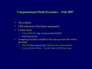
A bucket of water is poured through the air into a container of kerosene. This disrupts the kerosene, and air bubbles formed soon rise to the surface and break. The three liquids in this simulation do not mix, and after a time the water collects at the bottom of the container. The sliding mesh model is used to model the tipping of the bucket. Example: pouring water
Volume of fluid (VOF) model overview. VOF is an Eulerian fixed-grid technique. Interface tracking scheme. Application: modeling of gravity current. Surface tension and wall adhesion. Solution strategies. Summary. VOF Model
Lagrangian methods: The grid moves and follows the shape of the interface. Interface is specifically delineated and precisely followed. Suited for viscous, laminar flows. Problems of mesh distortion, resulting ininstability and internal inaccuracy. Eulerian methods: Fluid travels between cells of the fixed mesh and there is no problem with mesh distortion. Adaptive grid techniques. Fixed grid techniques, e.g. volume of fluid (VOF) method. Modeling techniques
Volume of fluid model • Immiscible fluids with clearly defined interface. • Shape of the interface is of interest. • Typical problems: • Jet breakup. • Motion of large bubbles in a liquid. • Motion of liquid after a dam break. • Steady or transient tracking of any liquid-gas interface. • Inappropriate if bubbles are small compared to a control volume (bubble columns).
VOF • Assumes that each control volume contains just one phase (or the interface between phases). • Solves one set of momentum equations for all fluids. • Surface tension and wall adhesion modeled with an additional source term in momentum equation. • For turbulent flows, single set of turbulence transport equations solved. • Solves a volume fraction conservation equation for the secondary phase.
Volume fraction • Defines a step function equal to unity at any point occupied by fluid and zero elsewhere such that: • For volume fraction of kth fluid, three conditions are possible: • k = 0 if cell is empty (of the kth fluid). • k = 1 if cell is full (of the kth fluid). • 0 < k < 1 if cell contains the interface between the fluids.
Volume fraction (2) • Tracking of interface(s) between phases is accomplished by solution of a volume fraction continuity equation for each phase: • Mass transfer between phases can be modeled by using a user-defined subroutine to specify a nonzero value for Sk. • Multiple interfaces can be simulated. • Cannot resolve details of the interface smaller than the mesh size.
Interface tracking schemes Donor-Acceptor Scheme Linear slope reconstruction Example of free surface
Comparing different interface tracking schemes 2nd order upwind. Interface is not tracked explicitly. Only a volume fraction is calculated for each cell. Donor - Acceptor Geometric reconstruction
Surface tension • Surface tension along an interface arises from attractive forces between molecules in a fluid (cohesion). • Near the interface, the net force is radially inward. Surface contracts and pressure increases on the concave side. • At equilibrium, the opposing pressure gradient and cohesive forces balance to form spherical bubbles or droplets.
Surface tension example • Cylinder of water (5 x 1 cm) is surrounded by air in no gravity. • Surface is initially perturbed so that the diameter is 5% larger on ends. • The disturbance at the surface grows by surface tension.
Surface tension - when important • To determine significance, first evaluate the Reynolds number. • For Re << 1, evaluate the Capillary number. • For Re >> 1, evaluate the Weber number. • Surface tension important when We >>1 or Ca<< 1. • Surface tension modeled with an additional source term in momentum equation.
Wall adhesion • Large contact angle (> 90°) is applied to water at bottom of container in zero-gravity field. • An obtuse angle, as measured in water, will form at walls. • As water tries to satisfy contact angle condition, it detaches from bottom and moves slowly upward, forming a bubble.
Modeling of the gravity current • Mixing of brine and fresh water. • 190K cells with hanging nodes. • Domain: length 1m, height 0.15m. • Time step: 0.002 s. • PISO algorithm. • Geometric reconstruction scheme. • QUICK scheme for momentum. • Run time ~8h on an eight-processor (Ultra2300) network. Brine: m=0.001 r=1005.1 Water: m=0.001 r=1000 g =9.8
Gravity current (1) T = 0 s T = 1 s T = 2 s
Gravity current (2) T = 3 s T = 4 s T = 5 s
Gravity current (3) T = 7 s T = 9 s T = 10 s
Visco-elastic fluids - Weissenberg effect • Visco-elastic fluids, such as dough and certain polymers, tend to climb up rotating shafts instead of drawing down a vortex. • This is called the Weissenberg effect and is very difficult to model. • The photograph shows the flow of a solution of polyisobutylene.
Blow molding is a commonly used technique to manufacture bottles, canisters, and other plastic objects. Important parameters to model are local temperature and material thickness. Visco-elastic fluids - blow molding
VOF model formulations - steady state • Steady-state with implicit scheme: • Used to compute steady-state solution using steady-state method. • More accurate with higher order discretization scheme. • Must have distinct inflow boundary for each phase. • Example: flow around ship’s hull.
Time-dependent with explicit schemes: Use to calculate time accurate solutions. Geometric linear slope reconstruction. Most accurate in general. Donor-acceptor. Best scheme for highly skewed hex mesh. Euler explicit. Use for highly skewed hex cells in hybrid meshes if default scheme fails. Use higher order discretization scheme for more accuracy. Example: jet breakup. Time-dependent with implicit scheme: Used to compute steady-state solution when intermediate solution is not important and the final steady-state solution is dependent on initial flow conditions. There is not a distinct inflow boundary for each phase. More accurate with higher order discretization scheme. Example: shape of liquid interface in centrifuge. VOF model formulations - time dependent
VOF solution strategies: time dependence • Time-stepping for the VOF equation: • Automatic refinement of the time step for VOF equation using Courant number C: • t is the minimum transit time for any cell near the interface. • Calculation of VOF for each time-step: • Full coupling with momentum and continuity (VOF updated once per iteration within each time-step): more CPU time, less stable. • No coupling (default): VOF and properties updated once per time step. Very efficient, more stable but less accurate for very large time steps.
VOF solution strategies (continued) • To reduce the effect of numerical errors, specify a reference pressure location that is always in the less dense fluid, and (when gravity is on) a reference density equal to the density of the less dense fluid. • For explicit formulations for best and quick results: • Always use geometric reconstruction or donor-acceptor. • Use PISO algorithm. • Increase all under-relaxation factors up to 1.0. • Lower timestep if it does not converge. • Ensure good volume conservation: solve pressure correction equation with high accuracy (termination criteria to 0.001 for multigrid solver). • Solve VOF once per time-step. • For implicit formulations: • Always use QUICK or second order upwind difference scheme. • May increase VOF under-relaxation from 0.2 (default ) to 0.5.
Summary • Free surface flows are encountered in many different applications: • Flow around a ship. • Blow molding. • Extrusion. • Mold filling. • There are two basic ways to model free surface flows: • Lagrangian: the mesh follows the interface shape. • Eulerian: the mesh is fixed and a local volume fraction is calculated. • The most common method used in CFD programs based on the finite volume method is the volume-of-fluid (VOF) model.