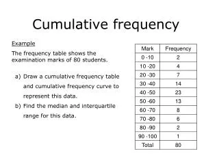
Download
1 / 32
320 likes | 435 Views
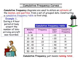
Statistical Properties of the Cumulative Frequency Diagram (CFD). ERF Conference, Nov. 2007 Elgin S. Perry, Statistics Consultant Paul T. Jacobson, Langhei Ecology, LLC Session: SCI-060, Abstract ID: 2419.

E N D
Statistical Properties of the Cumulative Frequency Diagram (CFD). ERF Conference, Nov. 2007 Elgin S. Perry, Statistics Consultant Paul T. Jacobson, Langhei Ecology, LLC Session: SCI-060, Abstract ID: 2419
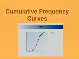
The Cumulative Frequency Diagram (CFD) is a novel tool for assessing the Pass/Fail of water quality criteria over space and time.
Poster Objectives • Motivate CFD • Define CFD • Give simple numerical example • Review CFD properties based on simple model of water quality • Review unresolved statistical issues concerning CFD
Motivation for CFD Assessment tool • Differentiate temporal and spatial variance in criteria assessment • Allow spatially broad but ephemeral events. • Allow spatially small but persistent events.
Steps to Compute a CFD • Set Compliance criteria, C, (C may be a collection of criteria that vary in time and space) • Collect k spatial samples over segment for m dates in assessment period. • For each date interpolate (e.g. Kriging) the k samples to n cells over segment.
4. Compute Area-based exceedences For each date estimate proportion of segment that does not comply with C.
5. Score Area-base exceedences across dates Rank from high to low the Area-based exceedences: psj. Score time dimension of each point proportional rank. Plot step ptj versus psj.
date1 date2 date3 Step 1. Collect data at known locations. Step 2. Interpolate data to grid cells. Step 3. Determine status of each cell.
Step 4: Percent compliance by date. Step 5. Rank the percent of space values assign percent of time = (100*R/(M+1))
Simple Example Plotted Fraction of Time Fraction of Space
Fig. 1 Simple example of CFD showing excessive violations of water quality relative to the reference curve.
Establishing Reference Curves • Use simple model to estimate curve based on 10% expected violations (theoretical curve). • Empirically estimate curve based on water quality in a reference area (empirical curve).
Reference Curves empirical curve for DO Based on benthic IBI > 3 theoretical curve based on 10% noncompliance
Fig 2. Examples of theoretical reference curve and empirical reference curve.
How is temporal and spatial variability of water quality reflected in shape of the CFD curve?Using a simple model and probability theory we can compute the theoretical CFD.
Simple Water Quality ModelXij = u + ai + bij i = 1, 2, . . . M and j = 1, 2, . . . N.a is temporal term, var =b is spatial term, var =
CFD as Mean Decreases Below C = 5. Fraction of Time Fraction of Space
Fig. 3. As the mean of water quality decreases from the criterion, the CFD retreats toward the origin of the Space-Time plane.
CFD as Temporal Variance Increases. Fraction of Time Fraction of Space
Fig. 4. As the temporal variance of water quality increases, the CFD deflects toward broad areas of space in noncompliance for a short time.
CFD as Spatial Variance Increases. Fraction of Time Fraction of Space
Fig. 5. As the spatial variance of water quality increases, the CFD deflects toward increasing areas of space persistently in noncompliance.
Statistical Issues • Current simulation exercises show that the shape of the CFD is influenced by level of sampling. As a result the estimated CFD is biased for the true CFD. • A confidence envelope for the CFD is analytically complex. This limits statistical inference.
Fraction of time Fraction of space
Fig. 6. Simulation shows that as sample size decreases, the estimated CFD deflects away from the true CFD. This is the result of increasing variability with decreasing sample size.
Fig. 7. Conditional simulation based on Kriging shows promise of correcting the sample size bias and providing a statistical inference too. Confidence bounds were computed based on quantiles of fraction of space computed on conditionally simulated surface estimates using variogram estimates from data.
Conclusion • The method show promise as a method for addressing temporally and spatially detailed criteria. • Sampling Bias and Statistical Inference issues need to be resolved.
See also: Jacobson, P.; Perry, E., Time-space Criteria for Water Quality in Chesapeake BaySession:SCI-060 - Innovations in Collection, Interpretation and Application of Monitoring DataTime & PlaceTuesday, 11:00 AM in 555 AB (RICC)
Futher Details: U.S.E.P.A. 2007. Ambient Water Quality Criteria for Dissolved Oxygen, Water Clarity and Chlorophyll a for the Chesapeake Bay and its Tidal Tributaries. 2007 Addendum. EPA 903-R-07-003. Region III Chesapeake Bay Program Office, Annapolis, Md. Secor, David, et al. (2006) Review of the Chesapeake Bay Program CFD and Interpolator. Chesapeake Bay Program’s Scientific and Technical Advisory Committee, Chesapeake Research Consortium, Edgewater, Md.http://www.chesapeake.org/stac/stacpubs.html#RR