Introductory tutorial to the RF Module: Coil design
450 likes | 617 Views
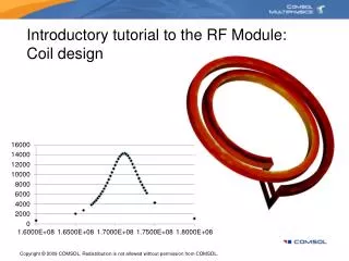
Introductory tutorial to the RF Module: Coil design. Introductory tutorial to the RF Module: Coil design. This coil has a resonant frequency at which the stored electric and magnetic energy are equal. At this frequency the coil stores energy very well.

Introductory tutorial to the RF Module: Coil design
E N D
Presentation Transcript
Introductory tutorial to the RF Module:Coil design This coil has a resonant frequency at which the stored electric and magnetic energy are equal. At this frequency the coil stores energy very well. We will find the resonant frequency and quantify how well the coil stores energy. We will then tune the resonant frequency and consider coupling to another coil.
Solution procedure: • Find the resonant frequency of the coil • Investigate the boundary conditions • Add surface losses • Determining the Q-factor • Tune the resonant frequency with lumped parameters • Scan over frequency • Add another coil
Open a new, blank, 3D RF model file and import the coil geometry
Add a surrounding air sphere and solve for the fields around, but not inside, the coil by deactivating the equations inside the coil Mesh, for now, with the “Extra Coarse” Setting
Use PEC boundaries on the coil surface and PMC boundaries on the sphere surface The PEC boundary condition models infinitely conductive media, with no losses, it sets the tangential component of the E-field to zero. Fields do not penetrate past the boundary. Incident wave E-field Loss-less out-of-phase reflected wave The PMC boundary condition models a symmetry boundary condition, the derivative of the tangential E-field is zero. Fields do not penetrate past the boundary. Loss-less in-phase reflected wave
Try solving the model… Solving for eigenvalues is an iterative process, the default is to start searching around a frequency of zero. This is “too far away” from the solution, and you will get an error message similar to the above… The resolution to this error message, or slow convergence, is to search around a different frequency
Tuning the solver… Enter 1 here, we are only interested in, the first resonant frequency, the fundamental mode Ramp this up by powers of 100 until a solution is returned. Once you get a solution, enter that as the new search point and go down in frequency by powers of 10, and then, by ½ to make sure that you have the fundamental mode. It is easiest to search from above, in frequency. Do so, if you roughly know the resonant frequency. The default PARDISO direct solver is the fastest for this type of problem. If you are running out of memory, use the PARDISO out-of-core option, or GMRES, but these are much slower.
When plotting results, remember that electric and magnetic fields are out of phase
Verify that this is the fundamental mode Slice plot of total energy density f = 178 MHz f = 1.74 GHz Numerically, there is no difference between the modes, the fundamental mode is simply the resonant mode closest to zero in frequency, but the eigenvalue solver will return whatever modes are closest to the given starting point
Spurious modes may be returned if you starting frequency is too low f = 2287 Hz These modes are numerically correct but have no physical meaning, they are an artifact of the finite element mesh
Enforcing the divergence condition will reduce the appearance of spurious modes Set this via: Physics > Application Mode Properties When enforcing the Divergence condition, you must use one of the direct solvers such as PARDISO This also increases the problem size, and memory requirements, so it is generally less attractive
Study increasing the air sphere radius, and switch the outside boundary conditions from PMC to PEC This is a fundamental result, the PMC and PEC boundary conditions can be though of as opposites, or as bounds to the problem. The mesh also has an effect upon this result Resonant Frequency, MHz Sphere radius
Tune the Free Mesh Parameters settings to get uniform aspect ratio elements around the coil Study the mesh refinement as discussed in the Dipole Antenna Tutorial
So far, the structure is loss-less, let us know consider skin losses on the coil surface Enter the conductivity of the coil
When solving this problem, an error occurs The eigenvalue problem solves for the resonant frequency, but the losses due to a finite conductivity boundary are a function of this resonant frequency. The problem is now a non-linear eigenvalue problem, and we must provide not just a starting point for the eigenvalue solver, but also a guess at the frequency for the conductive losses.
Use the loss-less eigenfrequency as the guess for the lossy calculation Use the linear eigenvalue solution, and multiply that by i and the frequency: -i*2*pi*1.78e8
This non-linear eigenvalue problem will take longer to solve, but will return the Q-factor Postprocessing > Data Display > Global This is the Q-factor due to resistive losses, usually there is only a small shift in resonant frequency
Use a PML to compute the radiative losses F = 171 MHz Qtotal = 35 See the dipole antenna tutorial for instructions on how to build this PML Solving with a PML will significantly increase solution time
It is also possible to get the resonant mode and Q-factor from a frequency sweep Add embedded surfaces to represent PEC faces (blue) and a Lumped Port (red) Switch to the Time-harmonic formulation to get access to the Lumped Port BC’s
Change the solver settings to scan over frequency Start with a coarse frequency scan Use the GMRES solver with all defaults. This solver is better for solving frequency domain problems, and uses much less memory.
Sometimes, an under-meshed PML can lead to extremely slow convergence The mesh under-resolves the fields, so the iterative solver cannot converge. The direct solvers will still work. Not enough elements here A well-resolved mesh will converge when using the iterative solver. Better convergence
Monitor port impedance and increase resolution on the frequency scan near the peak f0 Zmax Real(Z) ½ Zmax Δf Frequency
Q-factor can be computed two ways: Where f0 and Δf are found from the frequency scan U: Integral of stored energy in all domains P: Radiated power & surface losses (both evaluated at f0)
Now that we have the resonant frequency, we can tune the coil with lumped parameters Zcoil V Consider two strategies: Zcoil V Add some additional faces to model a circuit
Use Lumped Ports to add capacitance Zcapacitor= -j/ωC (ω=omega_rfw)
Re-run the frequency scan… Parallel Circuit Original Coil Q-factor does not change much, but the resonant frequency is shifted due to the added capacitance, and the impedance is lower for the series circuit. Real(Z) Series Circuit Frequency
Compute coupling to a second coil PEC Lumped Port The lumped port boundary conditions set up additional global output variables for port voltage: Vport_<port #>_g1_rfw and port current: Iport_<port #>_g1_rfw A coil need not have volume, create a loop of PEC faces, and a Lumped Port
What you should have learned… • Finding the resonant frequency of a loss-less, non-radiating coil • Adding resistive losses to the coil • Adding radiative losses • Finding the Q-factor • Tuning the resonant frequency via lumped ports • Computing the coupling to another coil
How to define a circuit port with a source current using the SPICE interface Zcoil Going back to the case with one tuning capacitance and just one coil. How do we define a current source rather than a voltage source? I
Change the boundary condition from Lumped port to Circuit Port. Keep the Port number set to 1.
When adding a Circuit port, COMSOL now considers the port to have two terminals. This fact will be used in the SPICE circuit definition.
SPICE Circuit 1 A • We will add a SPICE circuit corresponding to this circuit diagram. • It consists of one current source of 1 Amps , one impedance or 50 Ohm and a total of three circuit nodes named 0, 1 and 2. • The two Circuit Port terminals will correspond to the nodes 0 and 2. 1 0 Circuit port 50 Ohm 2
To add a current source, click the Create Current Source button. Give the device the name I1 (for current source 1). Let it have terminal names 0 and 1. Give the Device value the value 1 (this correspond to 1 Ampere).
To add a real impedance (resistor), click the Create Resistor button. Give the device the name R1 (for resistor 1). Let it have Terminal names 1 and 2. Give the Device value the value 50 (this correspond to 50 Ohm).
To add an external circuit – which will be the 3D coil model – click the Create Subcircuit Instance. Give the device the name X1 (for external circuit 1). Let it have Terminal names 2 and 0. Give the Subcircuit reference name rfcoil. This is your chosen name for the 3D coil model.
To add a link to the 3D coil model, click the Create Link to Current Model button. Give the Subcircuit reference name rfcoil (needs to match what’s given for X1). Set Terminal names to 1. Note: this is the port number of the circuit port in the 3D coil model and does not reference any of the SPICE nodes.
Now select the Force AC analysis checkbox. This will turn the circuit into an AC circuit (frequency-response/harmonic analysis).
Plot of port impedance (real and imaginary part) vs. frequency. These correspond to the variable expressions: Real part: real(Zport_1_rfw) or just Zport_1_rfw (Since COMSOL automatically takes the real part of all expressions plotted.) Imaginary part: imag(Zport_1_rfw)