Thermodynamic Control Volume
310 likes | 654 Views
Thermodynamic Control Volume. Build a simple model from scratch Based on physical principles Demonstrate typical model design trade off Simplicity vs range of validity Simplicity vs numerical robustness Dynamic vs static. Thermodynamic Control Volume.

Thermodynamic Control Volume
E N D
Presentation Transcript
Thermodynamic Control Volume • Build a simple model from scratch • Based on physical principles • Demonstrate typical model design trade off • Simplicity vs range of validity • Simplicity vs numerical robustness • Dynamic vs static
Thermodynamic Control Volume Control volume: First Law for Open Systems Connector: heat transfer Connector: convective flow M, U Mass- and Energy Balances
Step One: Connectors • Two transported quantities: mass & energy • flow variable • flow variable • Potential variable for mass flow: pressure • For bi-directional flow: specific enthalpy h
Step One: Connectors connector SimpleFlow SIunits.Pressure p; SIunits.SpecificEnthalpy h; flow SIunits.MassFlowRate mdot; flow SIunits.Power q_conv; end SimpleFlow;
Thermodynamic Control Volume Constitutive Laws: Ideal Gas Law
Ideal Gas Law partial model PureIdealGas "Ideal Gas Law" SIunits.SpecificHeatCapacity cv, cp, R; SIunits.SpecificEnergy u; SIunits.Temperature T; SIunits.Pressure p; SIunits.Volume V; SIunits.Mass M; equation p*V = M*R*T; cv = cp - R; u = cv*T; end PureIdealGas;
Thermodynamic Control Volume Constitutive Laws: physical properties for H2
Hydrogen Properties partial model H2cp "cp, for NASA coefficients" SIunits.SpecificHeatCapacity cp; SIunits.Temperature T(min=200, max=1000); // range of validity of polynomial replaceable IdealGasData data; equation cp = data.R*(1/(T*T)*(data.a[1] + T*(data.a[2] + T*(1.*data.a[3] + T*(data.a[4] + T*(data.a[5] + T*(data.a[6] + data.a[7]*T) )))))); end H2cp;
Boundary Conditions Given fixed inflow, Infinite Reservoir with fixed pressure at outflow Turbulent pressure drop
Boundary Conditions I model SimpleReservoir parameter SIunits.Temperature T0=300; parameter SIunits.Pressure p0=1.0e5; parameter SIunits.SpecificHeatCapacity cp0=H2cp_init(T0); FlowA a; equation a.p = p0; a.h = cp0*T0; end SimpleReservoir;
Boundary Conditions II model FlowSource parameter SIunits.MassFlowRate mdot_fix=1.0; parameter SIunits.Temperature T0=300; parameter SIunits.SpecificHeatCapacity cp0=H2cp_init(T0); FlowB b; equation b.mdot = -mdot_fix; b.q_conv = -mdot_fix*cp0*T0; end FlowSource;
Turbulent Flow Resistance model SimplePressureDrop parameter SIunits.Pressure dp0=1.0e3; parameter SIunits.MassFlowRate mdot0=0.1; FlowA a; FlowB b; protected SIunits.Pressure dp; equation dp = a.p - b.p; a.mdot = if dp > 0 then sqrt(dp/dp0) else -sqrt(-dp/dp0); a.q_conv = if dp > 0 then a.h*a.mdot else b.h*a.mdot; b.mdot = -a.mdot; b.q_conv = -a.q_conv; end SimplePressureDrop;
Turbulent Flow Resistance Will this model work for reversing flows?
Thermodynamic Control Volume Control volume: First Law for Open Systems Connector: heat transfer Connector: convective flow M, U Mass- and Energy Balances
Thermodynamic Control Volume model SimpleControlVolume parameter SIunits.Temperature T0=300.0; parameter SIunits.Pressure p0=1.0e5; parameter SIunits.Volume V0=1.0; extends H2(M(start=p0*V0/(data.R*T0)),T(start=T0)); SIunits.InternalEnergy U(start=p0*V0*(H2cp_init(T0) - data.R)/data.R); FlowA a; FlowB b; equation der(M) = a.mdot + b.mdot; der(U) = a.q_conv + b.q_conv; U = M*u; V = V0; a.p = p; b.p = p; a.h = cp*T; b.h = a.h; end SimpleControlVolume1;
The Modelica Model 1 to 1 representation of physical model
How to Structure the Code? • Reusable Code • Top level: physical objects • Separate: • Medium specific functions for hydrogen • Constitutive equations, the ideal gas law • Mass and energy balances • Functions or Classes?
Numerical Considerations • What kind of equation system do we get? • Probable difficulties with initial values? • Numerical robustness guaranteed?
Numerical Considerations • Case I: • Internal energy U and mass M are the states • Initial Values for mass and internal energy? Non-linear equation!
Numerical Considerations • Case II: • can we avoid the non-linear system of equations? • Function cp(T) is causing the problem Choose T as a State instead of U • Let Dymola do the rewriting
Thermodynamic Control Volume model SimpleControlVolume parameter SIunits.Temperature T0=300.0; parameter SIunits.Pressure p0=1.0e5; parameter SIunits.Volume V0=1.0; extends H2(M(start=p0*V0/(data.R*T0)),T(start=T0)); SIunits.InternalEnergy U; Real dT; FlowA a; FlowB b; equation der(M) = a.mdot + b.mdot; der(U) = a.q_conv + b.q_conv; U = M*u; V = V0; a.p = p; b.p = p; a.h = cp*T; b.h = a.h; dT = der(T); end SimpleControlVolume1;
Numerical Considerations • Case II: • What about initial values?Much easier with T as a State than with U!
Thermodynamic Control Volume model SimpleControlVolume parameter SIunits.Temperature T0=300.0; parameter SIunits.Pressure p0=1.0e5; parameter SIunits.Volume V0=1.0; extends H2(p(start=p0,fixed=true),T(start=T0,fixed=true)); SIunits.InternalEnergy U(fixed=false); Real dp, dT; FlowA a; FlowB b; equation der(M) = a.mdot + b.mdot; der(U) = a.q_conv + b.q_conv; U = M*u; V = V0; a.p = p; b.p = p; a.h = cp*T; b.h = a.h; dT = der(T); dp = der(p); end SimpleControlVolume1;
Numerical Considerations • Case III: • Eliminate the need for extra functions or calculations for initial conditions • Make pressure p and Temperature T the states • easy initial conditions • measurements available? System identification • Let Dymola do the rewriting again
Reversing Flows Consider this almost trivial system • Switch of Blower after 1 s • Control Volumes cools down due to heat loss
Reversing Flows • A system that handles reversing flows works • If the pressure drop is , the system will fail for numerical reasons • Why? Look at the numerical details
Reversing Flows: Demo • Open “SimpleExamples.mo” • run scripts BackFlow.mos, NoBackFlow.mos • Important details for start up simulations etc.
ThermoFlow Library Goals • Supply basic dynamic flow models • Take care of initialization • Consider numerical efficiency • General numerical robustness important • Allowing reversing flows a must • Basic set of physical properties
Conclusions • Easy to build physical models with Modelica • Start with basic conservation equations • Define connectors • Numerical aspects important for robustness • Use model Libraries!