Integration Relation for Control Volume
330 likes | 861 Views
Integration Relation for Control Volume. The Reynolds Transport Theorem Conservation of Mass. LAGRANGIAN & EULERIAN DESCRIPTIONS. Lagrangian Approach : Describe the fluid particle’s motion with time. The path of a particle : r(t) = x(t) i + y(t) j + z(t) k

Integration Relation for Control Volume
E N D
Presentation Transcript
Integration Relation for Control Volume The Reynolds Transport Theorem Conservation of Mass
LAGRANGIAN & EULERIAN DESCRIPTIONS • Lagrangian Approach: • Describe the fluid particle’s motion with time. • The path of a particle: r(t) = x(t) i + y(t) j + z(t) k • i, j, k: unit vectors • Velocity of a particle : V(t) = dr(t) / dt = u i + v j + w k • Eulerian Approach: • Imagine an array of windows in the flow field: Have information for the fluid particles passing each window for all time. • In this case, the velocity is function of the window position (x, y, z) and time. • u = f1 (x, y, z, t) v = f 2 (x, y, z, t) w = f 3 (x, y, z, t) • Eulerian approach is generally favored
CONTROL VOLUME APPROACH: • “Focusing on a volume in space & Considering the flow passing through the volume” • * It derives from the Eulerian description of fluid motion. • * It involves transforming the governing equations for a given mass (Lagrangian form) into the corresponding equations for mass passing through a volume in space (Eulerian form) • Mathematical equation needed for this transformation: • REYNOLDS TRANSPORT THEOREM
RATE OF FLOW • Volumetric Flow Rate: ∆Volume in the figure: = Length x Area = (V ∆t) x A Q = discharge [m3/s] V = average velocity [m/s] A = cross sectional area [m2 • Mass Flow Rate: • Mass of fluid passing a station per unit time [kg/s] • ρ = density [kg/m3]
RATE OF FLOW: Generalized equation forms Volumetric Flow Rate Differential discharge: Using concept of dot product: Mass Flow Rate
Mean Velocity By definition: • In laminar flow, the mean velocity • is half the centerline velocity. • In turbulent flow, velocity • profile is nearly flat so the mean • velocity is close to centerline • velocity. • REAL VELOCITY PROFILE: • Parabolic for laminar flow • Logarithmic for turbulent flow
Control Volume Approach • FLUID SYSTEM: Continuous mass of fluid, containing always the same fluid particles – The mass of a system is constant • CONTROL VOLUME (cv): Volume in space. – It can deform with time – It can move & rotate – The mass of control volume can changewith time • CONTROL SURFACE (cs): • Surface enclosing the control volume • or boundary of control volume
Control Volume Approach By definition, the mass of the system is constant, so The rate form of Continuity Principle:
Example • Considering a CV as shown in the earlier figure, atank with cross-sectional area of 10 m2 has an inflow of 7kg/s and an outflow of 5 kg/s. Find the rate at which the water level in the tank is changing. The volume of CV: V = Ah The mass in the CV: M cv = r V = r Ah The rate of change of mass in the CV: By the continuity equation, the rate of change of water elevation: = (7 - 5 ) / (1000 x10) = 0.0002 m/s
Reynolds Transport Theorem B (extensive property) of a system: proportional to the mass of the system (like m, mV, E) b (intensive property) : independent of system mass and obtained by [B/mass] The most general form: (Read excellent explanations at pages 133-138) B: extensive property b: intensive property t: time ρ:density V: volume V: velocity vector A: area vector b b Left side is Lagrangian form & represents the rate of change of property Bof the system Right side is Eulerian form & represents the rate change of property B in CV+ the net outflow of property B through the CS This equation is often called “control volume equation”
Reynolds Transport Theorem: Simplified form If the mass crossing the control surface occurs through a number of inlet and outlet ports, and the velocity density and intensive property b are uniformly distributed (constant) across each port; then Please see the text book for the alternative form of the above equation
Continuity Equation Derives from the conservation of mass which states the mass of the system is constant in Lagrangian form. (M sys = const) The Eulerian form is derived by applying Reynolds transport theorem. In this case, extensive property: B cv = M sys The corresponding intensive property: b = M sys / M sys = 1
Continuity Equation Since dM sys / dt = 0 The general form of continuity equation: = 0 Accumulation rate Net outflow rate of mass in CV + of mass through CS If the mass crosses the control surface through a number of inlet and exit ports, the continuity equation simplifies to
EXAMPLE 5.4: Since there is only one inlet and exit port, the continuity equation simplifies to Mass flow rate in : ρ V A = 1000 x 7 x 0.0025 = 17.5 kg/s Mass flow rate out: ρ Q = 1000 x 0.003 = 3 kg/s Continuity equation: Mass is accumulating in the tank at this rate!
EXAMPLE: (Problem 5.49) Referring the figure below, find the velocity of the liquid through the inlet. At a certain time, the surface level in the tank is 1 m and rising at the rate of 0.1 cm/s.
Continuity Equation for Flow in a Pipe • Steady Flow • CV is fixed to pipe walls • Volume of CV is const. • Mcv = const. Continuity Equation Incompressible flow valid for steady & unsteady incompressible flow
Cavitation Phenomenon that occurs when the fluid pressure is reduced to the local vapor pressure and boiling occurs. Vapor bubbles form in the liquid, grow and collapse; producing shock wave, noise & dynamic effects: . RESULT lessened performance & equipment failure ! Cavitation typically occurs at locations where the velocity is high. In case b, flow rate is higher
Cavitation damage examples Impeller of a centrifugal pump Spillway tunnel in a power dam