Understanding Quantitative Data: Histograms, Stem-and-Leaf Plots, and Dotplots
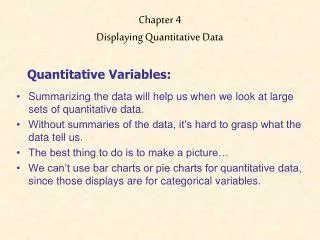
This chapter focuses on displaying quantitative data through histograms, stem-and-leaf plots, and dotplots. Histograms visualize data distribution using bins of equal intervals, with heights indicating frequency. The stem-and-leaf plot is an effective way to depict data with a key for clarity. Dotplots present individual data points along an axis for simplicity. The chapter also discusses data characteristics, including shape, center, and spread, emphasizing the importance of recognizing modes, symmetry, and outliers in your analysis.

Understanding Quantitative Data: Histograms, Stem-and-Leaf Plots, and Dotplots
E N D
Presentation Transcript
Chapter 4 Displaying Quantitative Data *histograms *stem-and-leaf plots *dotplot *shape, center, spread
Histogram • displays the distribution of QUANTITATIVE data in bins • the height of each bin represents the count of data values • bins have to have equal size intervals • there should be NO spaces between the bins
How to Make a Histogram • Slice up the entire span of values covered by the quantitative variable into equal width piles called bins (remember they need to be equal intervals) • Count the number of values that fall into each bin • data values that fall on the boarder of bins go in the higher bin • Be sure to label each axis (variable names and scales) • The bins and the count in each bin give the distribution of the quantitative variable
Stem-and-Leaf Plots Key: 5|3 = 5.3
Stem – and – Leaf Plots • Always make a key • Write numbers the same size and equally spaced (area principle) • More on stem-and-leaf plots coming Friday
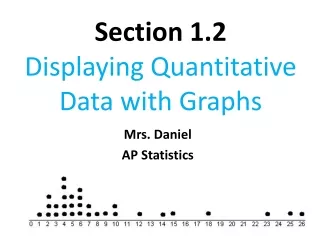
Dotplots • simple display • place a dot along an axis for each case in the data
Quantitative Data Condition • The data are values of a quantitative variable whose units are known • Always check before making a histogram, stem-and-leaf plot, or a dotplot
Describing Data • Shape: • how many bumps are there? • Bumps are called MODES (unimodal (1 bump), bimodal (2), multimodal ( > 3) • are there no bumps? Flat tops are called uniform • Is there symmetry? • symmetric – fold in half • skewed – tails to one side (skewed in that direction) • Any thing unusual? • outliers– any points that stand away from the rest of the data • gaps
Describing Data (cont) • Center • If you had to pick a single number to describe all the data • for now these are just estimates • Spread • Is the data tightly clustered around the center? • for now this will be described informally VARIATION MATTERS!!!!