Download

1 / 206
2.12k likes | 2.67k Views
The t Test In biology you often want to compare two sets of replicated measurements to see if they are the same or different. For example are plants treated with fertilizer taller than those without?

E N D
The t Test In biology you often want to compare two sets of replicated measurements to see if they are the same or different. For example are plants treated with fertilizer taller than those without? If the means of the two sets are very different, then it is easy to decide, but often the means are quite close and it is difficult to judge whether the two sets are the same or are significantly different. The t test compares two sets of data and tells you the probability (P) that the two sets are basically the same.
1.1.5 Deduce the significance of the difference between two sets of data using calculated values for t and the appropriate tables.(3) If you carry out a statistical significance test, such as the t-test, the result is a P value, where P is the probability that there is no difference between the two samples. A. When there is no difference between the two samples: A small difference in the results gives a higher P value, which suggests that there is no true difference between the two samples By convention, if P > 0.05 you can conclude that the result is not significant (the two samples are not significantly different).
B. When there is a difference between the two samples: A larger difference in results gives a lower P value, which makes you suspect there is a true difference (assuming you have a good sample size). By convention, if P < 0.05 you say the result is statistically significant. If P < 0.01 you say the result is highly significant and you can be more confident you have found a true effect. As always with statistical conclusions, you could be wrong! It is possible there really is no effect, and you had the bad luck to get sets of results that suggests a difference or not, where there is none.
Of course, even if results are statistically highly significant, it does not mean they are necessarily biologically important. Remember this when drawing conclusions. Correlation does not imply causation!
Causation and correlation ? 1.1.6 Explain that the existence of a correlation does not establish that there is a causal relationship between two variables.. Typically in Biology your experiment may involve a continuous independent variable and a continuously variable dependent variable. e.g effect of enzyme concentration on the rate of an enzyme catalyzed reaction. The statistical analysis would set out to test the strength of the relationship (correlation). Once a correlation between two factors has been established from experimental data it would be necessary to advance the research to determine what the causal relationship might be.
Causation It is important to realize that if the statistical analysis of data indicates a correlation between the independent and dependent variable this does not prove any causation. Only further investigation will reveal the causal effectbetween the two variables. Correlation does not imply causation! Skirt lengths and stock prices are highly correlated (as stock prices go up, skirt lengths get shorter). The number of cavities in elementary school children and vocabulary size have a strong positive correlation. Clearly there is no real interaction between the factors involved simply a co-incidence of the data.
Correlation vs. Causation :We have been discussing correlation. We have looked at situations where there exists a strong positive relationship between our variables x and y. However, just because we see a strong relationship between two variables, this does not imply that a change in one variable causes achange in the other variable. Correlation does not imply causation! Consider the following: In the 1990s, researchers found a strong positive relationship between the number of television sets per person x and the life expectancy y of the citizens in different countries. That is, countries with many TV sets had higher life expectancies. Does this imply causation? By increasing the number of TVs in a country, can we increase the life expectancy of their citizens? Are there any hidden variables that may explain this strong positive correlation?
There is a strong positive correlation between ice cream sales and shark attacks. That is, as ice cream sales increase, the number of shark attacks increase. Is it reasonable to conclude the following? Ice cream consumption causes shark attacks.
All of the previous examples show a strong positive correlation between the variables. However, in each example it is not the case that one variable causesa change in the other variable. For example, increasing the number of ice cream sales does not increase the number of shark attacks. There are outside factors, also known as lurking variables, which cause the correlation between these variables.
Correlation does not always mean that one thing causes the other thing (causation), because a something else might have caused both. For example, on hot days people buy ice cream, and people also go to the beach where some are eaten by sharks. There is a correlation between ice cream sales and shark attacks (they both go up as the temperature goes up in this case). But just because ice cream sales go up does not cause (causation) more shark attacks. Correlation does not imply causation!
You may be interested to know that global warming, earthquakes, hurricanes, and other natural disasters are a direct effect of the shrinking numbers of Pirates since the 1800s. For your interest, I have included a graph of the approximate number of pirates versus the average global temperature over the last 200 years. As you can see, there is a statistically significant inverse relationship between pirates and global temperature.
What is a t-test? A t-test is any statistical hypothesis test in which the test statistic follows a Student's t distribution if the null hypothesis is supported. What is a t-test used for? It can be used to determine if two sets of data are significantly different from each other, and is most commonly applied when the test statistic would follow a normal distribution.
The t-statistic was introduced in 1908 by William Sealy Gosset, a chemist working for the Guinness brewery in Dublin, Ireland ("Student" was his pen name). Gosset had been hired due to Claude Guinness's policy of recruiting the best graduates from Oxford and Cambridge to apply biochemistry and statistics to Guinness's industrial processes. Gosset devised the t-test as a cheap way to monitor the quality of stout.
The t-test work was submitted to and accepted in the journal Biometrika, the journal that Karl Pearson had co-founded and was the Editor-in-Chief; the article was published in 1908. Since Guinness had a company policy that chemists were not allowed to publish their findings, the company allowed Gosset to publish his mathematical work but only if he used a pseudonym, that was "Student".
How do you do a t-test? T-test values can be calculated with equations but we will calculate them using EXCEL. Type: 1or 2 Type 1: matched pairs Type 2: unpaired Number of tails: 1 or 2 df: degrees of freedom significance level ( ): usually P= 0.05
t-test to Compare Two Sample Means Student’s t-Test Student’s t-test is the most common (and simple) way of testing to see if there is a significant difference between two independent groups. The t-test statistic is calculated from the means, the number of samples in each group (n1 and n2), and the variance of each group (s1 and s2), according to the following equation. The variance is simply the standard deviation squared. Equation for t value for 2 means although you can use equations we will use EXCEL
T-Test using EXCEL Make data table in EXCEL Add cell P = Note: This only gives the P value Insert / Function / TTEST Array 1 Array 2 Type 1:paired Type 2:unpaired
You need to activate: Add ins: Data Analysis Toolpak
(1) Label a cell TTEST(2) Click on the adjacent cell (3) Tools | Data Analysis | T-test: Two-Sample Assuming equal variance
Hypothesis Testing Using t-tests What is Hypothesis Testing? Hypothesis testing is used to obtain information about a population parameter. A hypothesis is created about the population parameter, and then a sample from the population is collected and analyzed. The data found will either support or not support the hypothesis. A statistic is any value that is computed from the data in the sample. A test statistic is a statistic that can be used to find evidence in a hypothesis test. If a hypothesis test is conducted to find information about the population mean, the sample mean would be a logical choice of a statistic that would be useful.
Statistical test of difference using the t-Test. There are a few steps for evaluating a dataset or comparing multiple sets of data (statistical inference process). These steps are summarized here: list: 1. State the null hypothesis and the alternative hypothesis based on your research question. Define the hypothesis as to whether your means or standard deviations are significantly different. Null Hypothesis: 'There is no significant difference between the height of shells in sample A and sample B.' H0: μ = μ0 Alternative Hypothesis: 'There is a significant difference between the height of shells in sample A and sample B'. HA: μ ≠ μ0
Hypothesis Testing • The intent of hypothesis testing is formally examine two opposing conjectures (hypotheses), H0 and HA • These two hypotheses are mutually exclusive and exhaustive so that one is true to the exclusion of the other • We accumulate evidence - collect and analyze sample information - for the purpose of determining which of the two hypotheses is true and which of the two hypotheses is false
The Null and Alternative Hypothesis The null hypothesis, H0: • States the assumption (numerical) to be tested • Begin with the assumption that the null hypothesis is TRUE • Always contains the ‘=’ sign The alternative hypothesis, Ha: • Is the opposite of the null hypothesis • Challenges the status quo • Never contains just the ‘=’ sign • Is generally the hypothesis that is believed to be true by the researcher
Null and Alternative Hypotheses The null hypothesis, denoted H0, is the statement that is being tested. Usually the null hypothesis is the “status quo” or “no change” hypothesis. The hypothesis test looks for evidence against the null hypothesis. The alternative hypothesis, denoted HAor H1, is the statement that we are hoping is true or what we wish to prove. It is the “opposite” of the null hypothesis. Since we wish to prove the alternative hypothesis, we usually write the alternative hypothesis first and then the null hypothesis.
Statistical test of difference using the t-Test. 2. Set the critical P level (also called the alpha () level ) usually it will be P = 0.05 (5%) The p-value is the probability of observing an outcome as extreme or more extreme as the observed sample outcome if the null hypothesis is true. decide if the test should be 1- or 2-tailed determine the number of degrees of freedom. 3. Calculate the value of the appropriate statistic. Use the t-test for comparing means
Level of Significance Most hypothesis tests fall in the category of significance tests. Before the test is started (before the sample is chosen and anything is computed), a significance level, α is chosen. The most commonly used significance levels are α = 0.10, 0.05, or 0.01. If a significance level isn’t specified, α = 0.05 is the most common choice. The significance level is how much evidence is needed to reject the null hypothesis. For example, if α = 0.05 is chosen, the evidence is considered strong enough to reject the null hypothesis if the data in the sample would only happen 5% of the time, or less, when the null hypothesis is true. That means that the null hypothesis will only be rejected when the data in the sample isn’t very likely if the null hypothesis is true.
4. Write the decision rule for rejecting the null hypothesis. In biology the critical probability is usually taken as 0.05 (or 5%). This may seem very low, but it reflects the facts that biology experiments are expected to produce quite varied results. If P > 5% then the two sets are the same (i.e. accept the null hypothesis). If P < 5% then the two sets are different (i.e. reject the null hypothesis). For the t test to work, the number of repeats should be as large as possible, and certainly > 5.
5. Write a summary statement based on the decision. Example: The null hypothesis is rejected since calculated P = 0.003 < P = 0.05 two-tailed test Depending on whether the calculated value is greater than or less than the tabulated value, you accept or reject your hypothesis, and can thereby conclude whether your data is significantly different or not. 6. Write a statement of results in standard English. There is a significant difference between the height of shells in sample A and sample B.
What are degrees of freedom? The “df” in the t-distribution means “degrees of freedom”, in comparing 2 means
The t-distribution is a measure of the area under a curve. The normal distribution The central region on this graph is the acceptance area and the tail is the rejection region, or regions. In this particular graph of a two-tailed test, the rejection region is shaded blue. The tail is referred to as “alpha“, or p-value (probability value). The area in the tail can be described with z-scores. For example, if the area of the tails was 5% (2.5% each side).
The t-distribution looks almost identical to the normal distribution curve, only it’s a bit shorter and fatter. The t-distribution can be used for small samples. The larger the sample size, the more the t-distribution looks like the normal distribution. In fact, for sample sizes larger than 20, the t-distribution is almost exactly like the normal distribution. The “df” in the t-distribution means “degrees of freedom” and is just the sample size minus one (n-1).
This graph shows what three different t-distributions look like. With a larger sample size (black line, infinite degrees of freedom), the t-distribution looks identical to the normal curve. But with a smaller sample size of four (df = 3), the t-distribution curve is shorter and fatter.
How to Calculate a t-Distribution Step 1: Calculate the df, or degrees of freedom) . Step 2: Look up the df in the left hand side of the t-distribution table. Locate the column under your alpha level (the alpha level is usually given to you in the question. DF = 8
In general, statistical tests are used for comparing two means or two standard deviations to see if they are significantly different. You can also compare a mean from measured data to an accepted value to see if your sample measurements match the literature values.
There are two main types of t-tests we will use: The usual form of the t test is for "unmatched pairs" (type = 2), where the two sets of data are from different individuals. For example leaves grown in the sun and grown leaves in the shade.
The other form of the t test is for "matched pairs" (type = 1), where the two sets of data are from identical individuals. A good example of this is a ” before and after " test. For example the pulse rate of 8 individuals was measured before and after eating a large meal, with the results shown in the left. The mean pulse rate is certainly higher after eating, but is it significantly higher? Hint: type 1 has 1 group