Download

1 / 46
490 likes | 725 Views
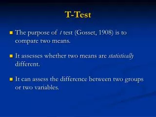
t-Test. Comparing Means From Two Sets of Data. Steps For Comparing Groups. Assumptions of t-Test. Dependent variables are interval or ratio. The population from which samples are drawn is normally distributed. Samples are randomly selected.

E N D
t-Test Comparing Means From Two Sets of Data
Assumptions of t-Test • Dependent variables are interval or ratio. • The population from which samples are drawn is normally distributed. • Samples are randomly selected. • The groups have equal variance (Homogeneity of variance). • The t-statistic is robust (it is reasonably reliable even if assumptions are not fully met.
Computing Confidence Intervals • We can determine the probability that a population mean lies between certain limits using a sample mean. • With inferential statistics we reverse this process and determine the probability that a random sample drawn from a specific population would differ by an observed result.
t Values • Critical value decreases if N is increased. • Critical value decreases if alpha is increased. • Differences between the means will not have to be as large to find sig if N is large or alpha is increased.
Probability that a sample came from a population? • Using the standard error we compute the probability that two means come from the same population. • If Z or t exceed the level of significance we conclude that the sample was • Not drawn from the population or • Has been modified so that it no longer represents the population
Relationship between t Statistic and Power • To increase power: • Increase the difference between the means. • Reduce the variance • Increase N • Increase α from α = .01 to α = .05
Does Volleyball Serve Training Improve Serving Ability? • Population mean = 31, sd = 7.5. • 30 students given serve training. Following training mean = 35, sd = 8.3. • Critical Z = 1.96 • Probability is greater than 99 to 1 that the mean did not come from original population. • The training was effective.
Volleyball Example Using t-statistic • Critical value of t(29)= 2.045, p = 0.05 • Since obtained t > critical value these means are statistical different.
Comparing Two Independent Samples • Independent samples (males, females), (swimmers, runners). • Must be different subjects in each group.
Independent t Test • If the t statistic is greater than the critical value we • Conclude the independent variable had a significant effect • And we reject chance as the cause of the mean difference.
Effects of Verbal Lesson of Basketball Shooting Skill Critical value of t(120) = 1.98, p = 0.05 Since our obtained t(98) = -1.36 is NOT greater than the critical value we ACCEPT the Null Hypothesis. The training had no effect upon shooting skill. Note: The sign +/- of t does not matter.
Does Positive Reinforcement Affect Bowling? Critical value t(40) = 2.201, p = 0.05 Since obtained t > critical t We reject the Null and state that positive reinforcement significantly improves bowling ability.
The t-test With Unequal N When you have unequal numbers of subjects in each group the statistic uses a different equation to estimate the standard error of the differences between groups.
The t-test With Unequal N Critical value of t(16) = 2.120, p = .05. The groups are significantly different.
Dependent or Paired t-test Note that the equation uses the correlation between pre and post samples. The Dependent t-test is more powerful that the Independent Groups t-test.
Dependent or Paired t-test The same subjects are in each group (DEPENDENT or PAIRED t-test). Critical value t(29) = 2.045, p = 0.05 The groups ARE SIGNIFICANTLY Different. Note: the correction formula adjusts the variance between groups. Since the same subjects are in each group you can expect less variance. Repeated Measures experiments are more powerful than independent groups
Does a Bicycle Tour Affect Self-Esteem?Are these differences MEANINGFUL???? Critical value of t(60) = 2.000, p = 0.05, so there is a significant difference. BUT DOES IT MEAN ANYTHING???
The Magnitude of the Difference (Size of Effect) • Omega squared can be used to determine the importance, or usefulness of the mean difference. • ω2 is the percentage of the variance (diff between means) that can be explained by the independent variable. • In this case the low-back and hip study explains 21% of variance between the means (pre & post).
Cohen’s Effect Size • Effect size of .2 is small, .5 moderate, .8 large • The control group is used to compute SD because it is not contaminated by the treatment effect.
The Percent Change is also useful in evaluating if a change is meaningful. • Before doing an experiment you should know what Percent Change would be considered meaningful. • For an Olympic athlete, a 1% (meaningful) improvement can be the difference between winning and losing. • For an untrained individual a 1% improvement would probably be meaningless.
Practical & Meaningful Significance • If two means are significantly different, that does not imply that they are practical. • If two means are NOT statistically significant, that does not imply that their differences are not practical. • Use ω2, Effect Size and Percent Change to evaluate the meaningfulness of an outcome.
Type I and Type II Errors Type I Error: Stating that there is a difference when there isn’t. Type II Error: Stating there is no difference when there is one.
We can never know if we have made a Type I or II error. • Statistics only provide the probability of making a Type I or II error. • The critical factor in this decision is the consequence of being wrong. • The confidence level should be set to protect against the most costly error. • Which is worse: to accept the null hypothesis when it is really false or to reject it when it is really true?
One Tail Test: Null A > B. More Powerful, easier to find differences.
Statistical Power • Power ( 1 - β ) depends upon: • Alpha [Zα (.10) = 1.65, Zα (.05) = 1.96] • Difference between the means. • Standard deviations between the two groups. • Sample size N.
To Increase Power • Increase alpha, Power for α = .10 is greater than power for α = .05 • Increase the difference between means. • Decrease the sd’s of the groups. • Increase N.
Calculation of Power From Table A.1 Zβ of .54 is 20.5% Power is 20.5% + 50% = 70.5% In this example Power (1 - β ) = 70.5%
Calculation of Sample Size to Produce a Given Power Compute Sample Size N for a Power of .80 at p = 0.05 The area of Zβ must be 30% (50% + 30% = 80%) From Table A.1 Zβ = .84 If the Mean Difference is 5 and SD is 6 then 22.6 subjects would be required to have a power of .80
Calculation of Sample Sized Need to Obtain a Desired Level of Power
Power • Research performed with insufficient power may result in a Type II error, • Or waste time and money on a study that has little chance of rejecting the null. • In power calculation, the values for mean and sd are usually not known beforehand. • Either do a PILOT study or use prior research on similar subjects to estimate the mean and sd.
Independent t-Test For an Independent t-Test you need a grouping variable to define the groups. In this case the variable Group is defined as 1 = Active 2 = Passive Use value labels in SPSS
Independent t-Test: Defining Variables Be sure to enter value labels. Grouping variable GROUP, the level of measurement is Nominal.
Independent t-Test: Output Assumptions: Groups have equal variance [F = .513, p =.483, YOU DO NOT WANT THIS TO BE SIGNIFICANT. The groups have equal variance, you have not violated an assumption of t-statistic. Are the groups different? t(18) = .511, p = .615 NO DIFFERENCE 2.28 is not different from 1.96
Dependent or Paired t-Test: Output Is there a difference between pre & post? t(9) = -4.881, p = .001 Yes, 4.7 is significantly different from 6.2