Transfer Functions
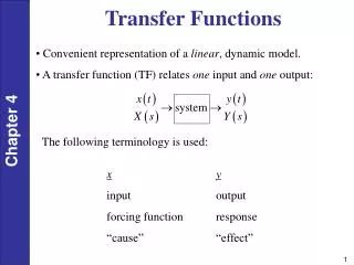
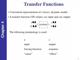
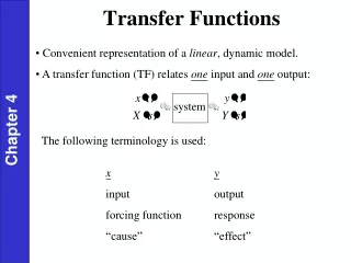
Transfer Functions. Convenient representation of a linear , dynamic model. A transfer function (TF) relates one input and one output:. The following terminology is used:. x input forcing function “cause”. y output response “effect”. Definition of the transfer function:

Transfer Functions
E N D
Presentation Transcript
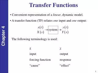
Transfer Functions • Convenient representation of a linear, dynamic model. • A transfer function (TF) relates one input and one output: The following terminology is used: x input forcing function “cause” y output response “effect”
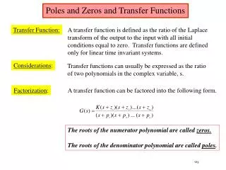
Definition of the transfer function: Let G(s) denote the transfer function between an input, x, and an output, y. Then, by definition where:
Development of Transfer Functions Example: Stirred Tank Heating System Figure 2.3 Stirred-tank heating process with constant holdup, V.
Recall the previous dynamic model, assuming constant liquid holdup and flow rates: Suppose the process is initially at steady state: where steady-state value of T, etc. For steady-state conditions: Subtract (3) from (1):
But, Thus we can substitute into (4-2) to get, where we have introduced the following “deviation variables”, also called “perturbation variables”: TakeLof (6):
Evaluate By definition, Thus at time, t = 0, But since our assumed initial condition was that the process was initially at steady state, i.e., it follows from (9) that Note: The advantage of using deviation variables is that the initial condition term becomes zero. This simplifies the later analysis. Rearrange (8) to solve for
where two new symbols are defined: Transfer Function Between and Suppose is constant at the steady-state value. Then, Then we can substitute into (10) and rearrange to get the desired TF:
Transfer Function Between and Suppose that Q is constant at its steady-state value: Thus, rearranging • Comments: • The TFs in (12) and (13) show the individual effects of Q and on T. What about simultaneous changes in both Q and ?
Answer: See (10). The same TFs are valid for simultaneous changes. • Note that (10) shows that the effects of changes in both Q and are additive. This always occurs for linear, dynamic models (like TFs) because the Principle of Superposition is valid. • The TF model enables us to determine the output response to any change in an input. • Use deviation variables to eliminate initial conditions for TF models.
Properties of Transfer Function Models • Steady-State Gain • The steady-state of a TF can be used to calculate the steady-state change in an output due to a steady-state change in the input. For example, suppose we know two steady states for an input, u, and an output, y. Then we can calculate the steady-state gain, K, from: For a linear system, K is a constant. But for a nonlinear system, K will depend on the operating condition
Calculation of K from the TF Model: If a TF model has a steady-state gain, then: • This important result is a consequence of the Final Value Theorem • Note: Some TF models do not have a steady-state gain (e.g., integrating process in Ch. 5)
Order of a TF Model • Consider a general n-th order, linear ODE: Take L, assuming the initial conditions are all zero. Rearranging gives the TF:
Definition: The order of the TF is defined to be the order of the denominator polynomial. Note: The order of the TF is equal to the order of the ODE. Physical Realizability: For any physical system, in (4-38). Otherwise, the system response to a step input will be an impulse. This can’t happen. Example:
G1(s) Y(s) G2(s) • Additive Property • Suppose that an output is influenced by two inputs and that the transfer functions are known: Then the response to changes in both and can be written as: The graphical representation (or block diagram) is: U1(s) U2(s)
Multiplicative Property • Suppose that, Then, Substitute, Or,
Linearization of Nonlinear Models • So far, we have emphasized linear models which can be transformed into TF models. • But most physical processes and physical models are nonlinear. • But over a small range of operating conditions, the behavior may be approximately linear. • Conclude: Linear approximations can be useful, especially for purpose of analysis. • Approximate linear models can be obtained analytically by a method called “linearization”. It is based on a Taylor Series Expansion of a nonlinear function about a specified operating point.
Linearization (continued) • Consider a nonlinear, dynamic model relating two process variables, u and y: Perform a Taylor Series Expansion about and and truncate after the first order terms, where , , and subscipt s denotes the steady state, Note that the partial derivative terms are actually constants because they have been evaluated at the nominal operating point, s.
Linearization (continued) Substitute (4-61) into (4-60) gives: Because is a steady state, it follows from (4-60) that
Example: Liquid Storage System Mass balance: Valve relation: A = area, Cv = constant Combine (1) and (2) and rearrange:
State-Space Models • Dynamic models derived from physical principles typically • consist of one or more ordinary differential equations (ODEs). • In this section, we consider a general class of ODE models referred to as state-space models. • Consider standard form for a linear state-space model,
where: • x = the state vector • u = the control vector of manipulated variables (also called control variables) • d = the disturbance vector • y = the output vector of measured variables. (We use boldface symbols to denote vector and matrices, and plain text to represent scalars.) • The elements of x are referred to as state variables. • The elements of y are typically a subset of x, namely, the state variables that are measured. In general, x, u, d, and y are functions of time. • The time derivative of x is denoted by • Matrices A, B, C, and E are constant matrices.
Example: CSTR Model Consider the previous CSTR model. Assume that Tccan vary with time while cAi, Ti, q and w are constant. Nonlinear Model: Linearized Model: where:
Example 4.9 • Show that the linearized CSTR model of Example 4.8 can • be written in the state-space form of Eqs. 4-90 and 4-91. • Derive state-space models for two cases: • Both cA and T are measured. • Only T is measured. Solution The linearized CSTR model in Eqs. 4-84 and 4-85 can be written in vector-matrix form:
Let and , and denote their time derivatives by and . Suppose that the coolant temperature Tc can be manipulated. For this situation, there is a scalar control variable, , and no modeled disturbance. Substituting these definitions into (4-92) gives, which is in the form of Eq. 4-90 with x = col [x1, x2]. (The symbol “col” denotes a column vector.)
If both T and cA are measured, then y = x, and C = I in Eq. 4-91, where I denotes the 2x2 identity matrix. A and B are defined in (4-93). • When only T is measured, output vector y is a scalar, and C is a row vector, C = [0,1]. Note that the state-space model for Example 4.9 has d= 0 because disturbance variables were not included in (4-92). By contrast, suppose that the feed composition and feed temperature are considered to be disturbance variables in the original nonlinear CSTR model in Eqs. 2-60 and 2-64. Then the linearized model would include two additional deviation variables, and .