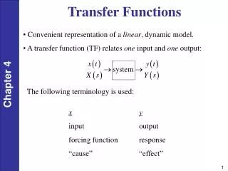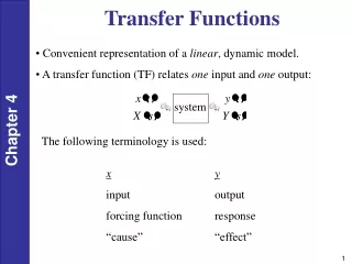
Transfer Functions
Transfer Functions. Professor Walter W. Olson Department of Mechanical, Industrial and Manufacturing Engineering University of Toledo. Outline of Today’s Lecture. A new way of representing systems Derivation of the gain transfer function Coordinate transformation effects

Transfer Functions
E N D
Presentation Transcript
Transfer Functions Professor Walter W. Olson Department of Mechanical, Industrial and Manufacturing Engineering University of Toledo
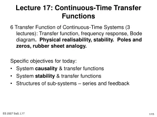
Outline of Today’s Lecture • A new way of representing systems • Derivation of the gain transfer function • Coordinate transformation effects • hint: there are none! • Development of the Transfer Function from an ODE • Gain, Poles and Zeros
Observability • Can we determine what are the states that produced a certain output? • Perhaps • Consider the linear system We say the system is observable if for any time T>0 it is possible to determine the state vector, x(T), through the measurements of the output, y(t), as the result of input, u(t), over the period between t=0 and t=T.
Observers / Estimators Input u(t) Output y(t) Noise State Observer/Estimator
Testing for Observability • For x(0) to be uniquely determined, the material in the parens must exist requiring to have full rank, thus also being invertible, the common test • Wo is called the Observability Matrix
Testing for Observability • For x(0) to be uniquely determined, the material in the parens must exist requiring to have full rank, thus also being invertible, the common test • Wo is called the Observability Matrix
Example: Inverted Pendulum • Determine the observabilitypf the Segway system with v as the output
Observable Canonical Form • A system is in Observable Canonical Form if it can be put into the form Where ai are the coefficients of the characteristic equation … u bn bn-1 b2 b1 D y z2 zn zn-1 … z1 S S S S S an an-1 a2 a1 -1 …
Observers / Estimators Output y(t) Input u(t) y + + B L A B C C A u Noise _ + + + + + Observer/Estimator State
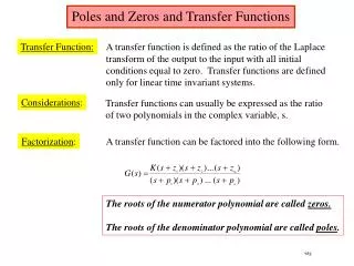
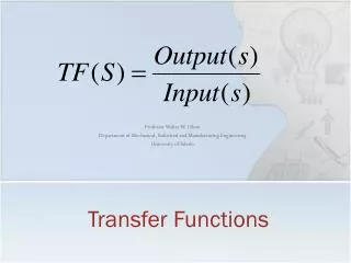
Alternative Method of Analysis • Up to this point in the course, we have been concerned about the structure of the system and discribed that structure with a state space formulation • Now we are going to analyze the system by an alternative method that focuses on the inputs, the outputs and the linkages between system components. • The starting point are the system differential equations or difference equations. • However this method will characterize the process of a system block by its gain, G(s), and the ratio of the block output to its input. • Formally, the transfer function is defined as the ratio of the Laplace transforms of the Input to the Output:
System Response From Lecture 11 • We derived for } } Steady State Transient Transfer function is defined as
Derivation of Gain • Consider an input of The first term is the transient and dies away if A is stable.
Example b k m x u(t)
Example b k m x u(t)
Coordination Transformations • Thus the Transfer function is invariant under coordinate transformation x1 z2 x2 z1
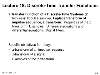
Linear System Transfer Functions General form of linear time invariant (LTI) system is expressed: For an input of u(t)=estsuch that the output is y(t)=y(0)est Note that the transfer function for a simple ODE can be written as the ratio of the coefficients between the left and right sides multiplied by powers of s The order of the system is the highest exponent of s in the denominator.
A DifferentMethod • Design a controller that will control the angular position to a given angle, q0
A DifferentMethod • Design a controller that will control the angular position to a given angle, q0
A DifferentMethod • Design a controller that will control the angular position to a given angle, q0 R=0.2 J= 10^-5 K=6*10^-5 Kb=5.5*10^-2 b=4*10^-2 gs=(K/(J*R))/(b*s^2/J+K*Kb*s/(J*R)) step(gs) Which was the same for the state space Later, we will learn how to control it
Gain, Poles and Zeros • The roots of the polynomial in the denominator, a(s), are called the “poles” of the system • The poles are associated with the modes of the system and these are the eigenvalues of the dynamics matrix in a state space representation • The roots of the polynomial in the numerator, b(s) are called the “zeros” of the system • The zeros counteract the effect of a pole at a location • The value of G(s) is the zero frequency or steady state gain of the system
Summary • A new way of representing systems • The transfer function • Derivation of the gain transfer function • Coordinate transformation effects • hint: there are none! • Development of the Transfer Function from an ODE • Gain, Poles and Zeros Next: Block Diagrams