Linear Circuit Analysis Through Transfer Functions
300 likes | 381 Views
Review the characteristics and analysis of linear time-invariant (LTI) systems using transfer functions in circuit analysis. Learn about impedance, admittance, power flow, and gain calculations. Explore examples and applications like noise filtering and filter design. No differential equations needed!

Linear Circuit Analysis Through Transfer Functions
E N D
Presentation Transcript
Lecture 2: Transfer Functions Prof. Niknejad
Review of LTI Systems • Since most periodic (non-periodic) signals can be decomposed into a summation (integration) of sinusoids via Fourier Series (Transform), the response of a LTI system to virtually any input is characterized by the frequency response of the system: Phase Shift Any linear circuit With L,C,R,M and dep. sources Amp Scale University of California, Berkeley
“Proof” for Linear Systems • For an arbitrary linear circuit (L,C,R,M, and dependent sources), decompose it into linear sub-operators, like multiplication by constants, time derivatives, or integrals: • For a complex exponential input x this simplifies: University of California, Berkeley
“Proof” (cont.) • Notice that the output is also a complex exp times a complex number: • The amplitude of the output is the magnitude of the complex number and the phase of the output is the phase of the complex number University of California, Berkeley
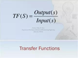
Complex Transfer Function • Excite a system with an input voltage (current) x • Define the output voltage y (current) to be any node voltage (branch current) • For a complex exponential input, the “transfer function” from input to output: • We can write this in canonical form as a rational function: University of California, Berkeley
+ – Arbitrary LTI Circuit Impede the Currents ! • Suppose that the “input” is defined as the voltage of a terminal pair (port) and the “output” is defined as the current into the port: • The impedanceZ is defined as the ratio of the phasor voltage to phasor current (“self” transfer function) University of California, Berkeley
+ – Arbitrary LTI Circuit Admit the Currents! • Suppose that the “input” is defined as the current of a terminal pair (port) and the “output” is defined as the voltage into the port: • The admmittanceZ is defined as the ratio of the phasor current to phasor voltage (“self” transfer function) University of California, Berkeley
+ – + – Arbitrary LTI Circuit Voltage and Current Gain • The voltage (current) gain is just the voltage (current) transfer function from one port to another port: • If G > 1, the circuit has voltage (current) gain • If G < 1, the circuit has loss or attenuation University of California, Berkeley
+ – + – Arbitrary LTI Circuit Transimpedance/admittance • Current/voltage gain are unitless quantities • Sometimes we are interested in the transfer of voltage to current or vice versa University of California, Berkeley
Power Flow • The instantaneous power flow into any element is the product of the voltage and current: • For a periodic excitation, the average power is: • In terms of sinusoids we have University of California, Berkeley
Power Flow with Phasors • Note that if , then • Important: Power is a non-linear function so we can’t simply take the real part of the product of the phasors: • From our previous calculation: Power Factor University of California, Berkeley
More Power to You! • In terms of the circuit impedance we have: • Check the result for a real impedance (resistor) • Also, in terms of current: University of California, Berkeley
Direct Calculation of H (no DEs) • To directly calculate the transfer function (impedance, transimpedance, etc) we can generalize the circuit analysis concept from the “real” domain to the “phasor” domain • With the concept of impedance (admittance), we can now directly analyze a circuit without explicitly writing down any differential equations • Use KVL, KCL, mesh analysis, loop analysis, or node analysis where inductors and capacitors are treated as complex resistors University of California, Berkeley
LPF Example: Again! • Instead of setting up the DE in the time-domain, let’s do it directly in the frequency domain • Treat the capacitor as an imaginary “resistance” or impedance: • Last lecture we calculated the impedance: → time domain “real” circuit frequency domain “phasor” circuit University of California, Berkeley
LPF … Voltage Divider • Fast way to solve problem is to say that the LPF is really a voltage divider University of California, Berkeley
Bigger Example (no problem!) • Consider a more complicated example: University of California, Berkeley
Does it sound better? • Application of LPF: Noise Filter • Listen to the following sound file (voice corrupted with noise) • Since the noise has a flat frequency spectrum, if we LPF the signal we should get rid of the high-frequency components of noise • The filter cutoff frequency should be above the highest frequency produced by the human voice (~ 5 kHz). • A high-pass filter (HPF) has the opposite effect, it amplifies the noise and attenuates the signal. University of California, Berkeley
Building Tents: Poles and Zeros • For most circuits that we’ll deal with, the transfer function can be shown to be a rational function • The behavior of the circuit can be extracted by finding the roots of the numerator and deonminator • Or another form (DC gain explicit) University of California, Berkeley
Poles and Zeros (cont) “poles” • The roots of the numerator are called the “zeros” since at these frequencies, the transfer function is zero • The roots of the denominator are called the “poles”, since at these frequencies the transfer function peaks (like a pole in a tent) University of California, Berkeley
Finding the Magnitude (quickly) • The magnitude of the response can be calculated quickly by using the property of the mag operator: • The magnitude at DC depends on G0 and the number of poles/zeros at DC. If K > 0, gain is zero. If K < 0, DC gain is infinite. Otherwise if K=0, then gain is simply G0 University of California, Berkeley
Finding the Phase (quickly) • As proved in HW #1, the phase can be computed quickly with the following formula: • No the second term is simple to calculate for positive frequencies: • Interpret this as saying that multiplication by j is equivalent to rotation by 90 degrees University of California, Berkeley
Bode Plots • Simply the log-log plot of the magnitude and phase response of a circuit (impedance, transimpedance, gain, …) • Gives insight into the behavior of a circuit as a function of frequency • The “log” expands the scale so that breakpoints in the transfer function are clearly delineated • In EECS 140, Bode plots are used to “compensate” circuits in feedback loops University of California, Berkeley
Example: High-Pass Filter • Using the voltage divider rule: University of California, Berkeley
40 dB 20 dB 0 dB -20 dB 20 dB 0.1 1 10 100 HPF Magnitude Bode Plot • Recall that log of product is the sum of log Increase by 20 dB/decade Equals unity at breakpoint University of California, Berkeley
0 dB -20 dB/dec ~ -3dB 0 dB -20 dB -40 dB -60 dB 20 dB HPF Bode Plot (dissection) • The second term can be further dissected: - 3dB University of California, Berkeley
0 dB -20 dB -40 dB Composite Plot • Composit is simply the sum of each component: High frequency ~ 0 dB Gain Low frequency attenuation University of California, Berkeley
Approximate versus Actual Plot • Approximate curve accurate away from breakpoint • At breakpoint there is a 3 dB error University of California, Berkeley
-45 Actual curve -90 HPF Phase Plot • Phase can be naturally decomposed as well: • First term is simply a constant phase of 90 degrees • The second term is a classic arctan function • Estimate argtan function: University of California, Berkeley